![]() Linear electrical circuits consist of resistors, capacitors, inductors, and voltage
and current sources. Let us consider here a simple resistor-inductor (RL)
one-port network driven by a current source. When a current I = I(t) is
applied to the input port, the voltage V = V(t) develops
across the port terminals. The voltage output V(t) can be determined as a sum of
the voltage drop across the resistor (which is R I(t) from the Ohm's law)
and of the voltage drop across the inductor (which is L I'(t), where
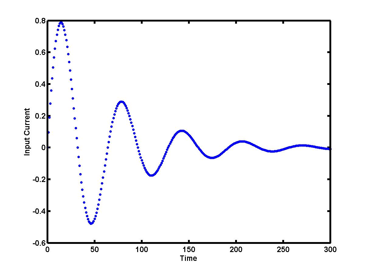
I'(t) denotes the derivative of I(t)). Suppose the input
current I(t) can be measured (detected) at different times t = tk
and it is generated by the following oscillatory and decaying signal
(click to enlarge the image):
Linear electrical circuits consist of resistors, capacitors, inductors, and voltage
and current sources. Let us consider here a simple resistor-inductor (RL)
one-port network driven by a current source. When a current I = I(t) is
applied to the input port, the voltage V = V(t) develops
across the port terminals. The voltage output V(t) can be determined as a sum of
the voltage drop across the resistor (which is R I(t) from the Ohm's law)
and of the voltage drop across the inductor (which is L I'(t), where
I'(t) denotes the derivative of I(t)). Suppose the input
current I(t) can be measured (detected) at different times t = tk
and it is generated by the following oscillatory and decaying signal
(click to enlarge the image):
The output voltage V(t) = R I(t) + L I'(t) can be computed at the times t = tk only if the derivative I'(tk) can be estimated numerically from the given data set (tk,Ik). This is the problem of numerical differentiation.
Let us denote the current time instance as t = t0, when the current is I = I0. Then, the data values in the past are: (t-1,I-1), (t-2,I-2), and so on. The data values in the future are: (t1,I1), (t2,I2), and so on. Depending on whether we use data in the future or in the past or both, the numerical derivatives can be approximated by the forward, backward and central differences. The simplest way to approximate the numerical derivatives is to look at the slope of the secant line that passes through two points (linear interpolation).
Consider a linear interpolation between the current data value (t0,I0) and the future data value (t1,I1). The slope of the secant line between these two points approximates the derivative by the forward (two-point) difference:
I'(t0) = (I1-I0) / (t1 - t0)
Forward differences are useful in solving ordinary differential equations by single-step predictor-corrector methods (such as Euler and Runge-Kutta methods). For instance, the forward difference above predicts the value of I1 from the derivative I'(t0) and from the value I0. If the data values are equally spaced with the step size h, the truncation error of the forward difference approximation has the order of O(h).
Consider a linear interpolation between the current data value (t0,I0) and the past data value (t-1,I-1). The slope of the secant line between these two points approximates the derivative by the backward (two-point) difference:
I'(t0) = (I0-I-1) / (t0 - t-1)
Backward differences are useful for approximating the derivatives if data in the future are not yet available. Moreover, data in the future may depend on the derivatives approximated from the data in the past (such as in control problems). If the data values are equally spaced with the step size h, the truncation error of the backward difference approximation has the order of O(h) (as bad as the forward difference approximation).
Finally, consider a linear interpolation between the past data value (t-1,I-1) and the future data value (t1,I1). The slope of the secant line between these two points approximates the derivative by the central (three-point) difference:
I'(t0) = (I1-I-1) / (t1 - t-1)
If the data values are equally spaced, the central difference is an average of the forward and backward differences. The truncation error of the central difference approximation is order of O(h2), where h is the step size. It is clear that the central difference gives a much more accurate approximation of the derivative compared to the forward and backward differences. Central differences are useful in solving partial differential equations. If the data values are available both in the past and in the future, the numerical derivative should be approximated by the central difference.
![]()