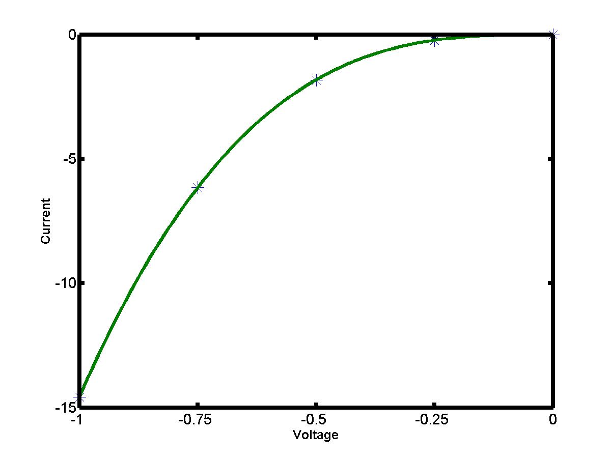
Here we apply the polynomial (Lagrange or Newton) interpolation algorithm to the given data values of a voltage-current characteristic of a zener diode (see figure again). Let us start with a few data values for negative voltages (where the voltage-current characteristic looks like a quadratic function):
| Voltage | -1.0000 | -0.7500 | -0.5000 | -0.2500 | 0.0000 |
|---|---|---|---|---|---|
| Current | -14.5773 | -6.1498 | -1.8222 | -0.2278 | 0.0000 |
We call the MATLAB function "LagrangeInter" (download the file and try it in MATLAB Command Window) for the Lagrange interpolation or the MATLAB function "NewtonInter" (download the file) for the Newton interpolation. In either the case, we obtain the following output (click the image to enlarge):
The interpolating polynomial has degree four for five data points. The polynomial interpolation is very good here because the graph resembles a lower-order polynomial. However, what if we want to interpolate the voltage-current characteristics for intermediate ranges, e.g. for data values:
| Voltage | -1.0000 | 0.0000 | 1.2750 | 2.5500 | 3.8250 | 4.9215 | 5.0235 |
|---|---|---|---|---|---|---|---|
| Current | -14.5773 | 0.0000 | 0.0000 | 0.0000 | 0.0000 | 0.8791 | 11.1683 |
In this case, the polynomial interpolation is not too good because of large swings of the interpolating polynomial between the data points:
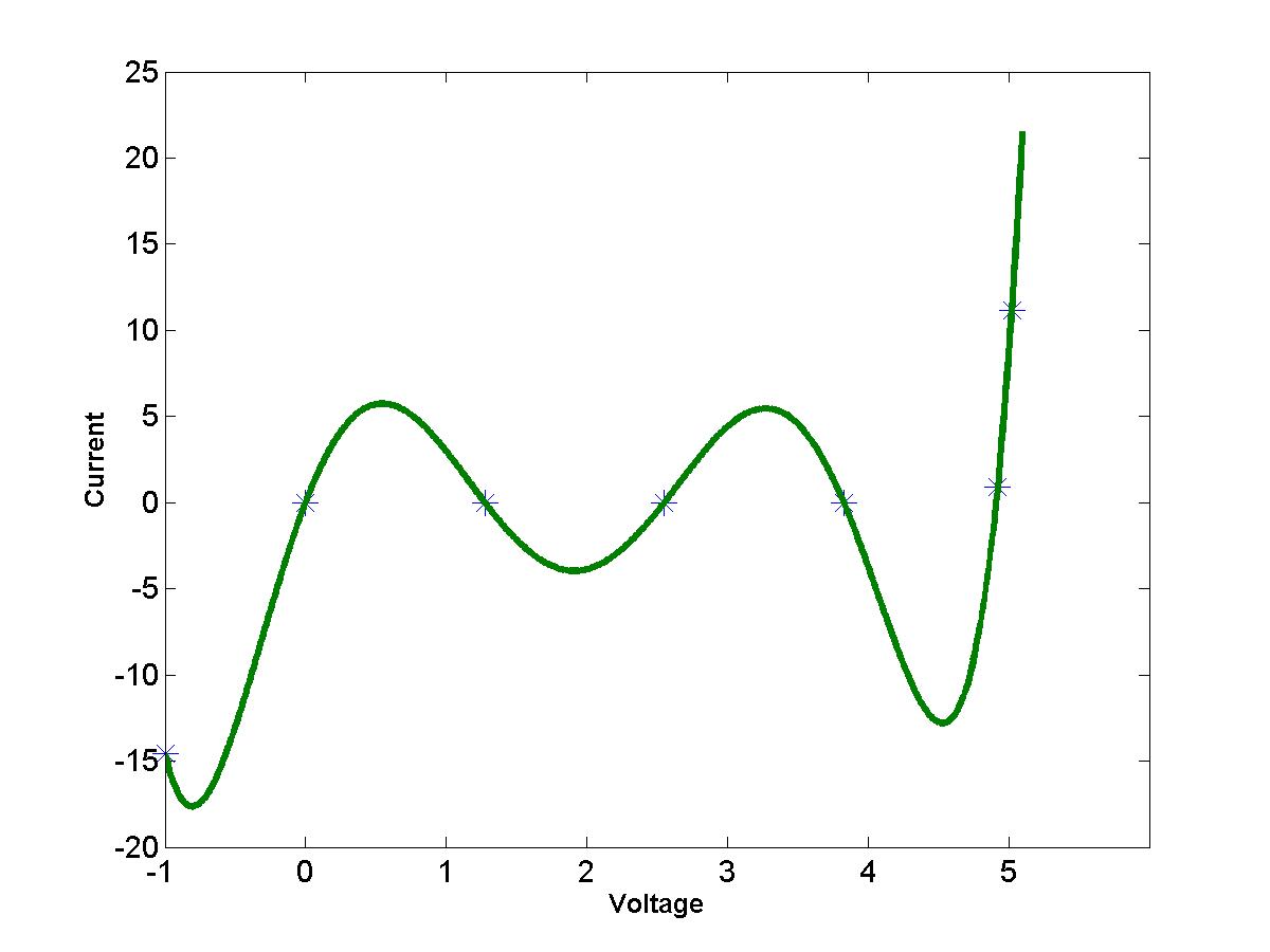
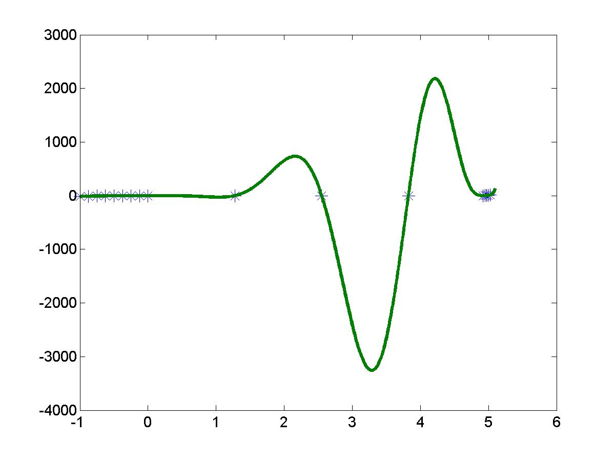
The interpolating polynomial has degree six for the intermediate data values and may have five extremal points (maxima and minima). Indeed, all five extrema show up in this polynomial interpolation leading to a polynomial wiggle. Let us finally take into account all given data: 18 data values. The polynomial interpolation shown below is really awkward: the error is so huge that the interpolating polynomial has nothing in common compared to the original voltage-current characteristic. Thus, the polynomial wiggle make appearance of higher-order polynomials unacceptable for data interpolation.