CHAPTER 4: MATHEMATICAL MODELING WITH MATLAB
Lecture 4.4: Root finding
algorithms for nonlinear equations
Problem: Given a nonlinear equation:
f(x) = 0
Find
all zeros (roots) x = x* of the function f(x).
Example:
Consider a
tunnel diode that has the following voltage (V) - current (I)
characteristics:
I = I(V) = V3 -
1.5 V2 + 0.6 V
The
tunnel diode is connected with a resistor (R) and a voltage
source (E). Applying the Kirchhoff's voltage law, one can find
that the steady current through the diode must satisfy the equation:
I(V) = ( E - V ) / R
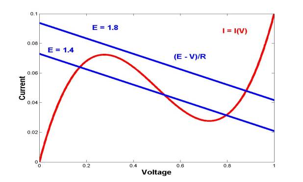
For given values of E
and R, this equation is of the form f(x) = 0, where
the voltage x = V is to be found. Graphing I = I(V) and
I = (E-V)/R at the same graph, one can show that either three or one
solutions are possible. Actual computations of the roots (zeros) are based on
the root finding algorithms.
% simple
example of root finding algorithms for polynomial functions
R = 19.2; E = 1.4; c = [ 1,-1.5,0.6+1/R,-E/R];
% coefficients of the
polynomial function f(x) = 0
p = roots(c)' % three steady currents throguh the tunnel
diode
E = 1.8; c = [ 1,-1.5,0.6+1/R,-E/R]; p = roots(c)' % one (real) steady current
p = 0.8801 0.3099 - 0.1023i 0.3099 + 0.1023i
Methods
of solution:
·
Bracketing
(bisection) methods
·
Iterative
(contraction mapping, Newton-Raphson, and secant) methods
·
MATLAB
root finding algorithms
Iterative
(contraction mapping) method:
Construct
the following mapping from xk to xk+1:
xk+1 = g(xk)
= xk + f(xk)
Starting
with an initial approximation x0, use the mapping
above to find x1, x2, etc. If
the sequence {xk} converges to a fixed point x =
x* such that x* = g(x*) = x*
+ f(x*), then the value x* is
the root (zero) of the nonlinear equation f(x) = 0.
% Graphical
solution of the nonlinear equation: x*sin(1/x) = 0.2*exp(-x)
x = 0.0001 : 0.0001 : 2; f1 = x.*sin(1./x); f2 = 0.2*exp(-x); plot(x,f1,'b',x,f2,'g');
% Contraction
mapping method for finding the root of the nonlinear equation:
% f(x) = x*sin(1/x)-0.2*exp(-x)
x = 0.364; % starting approximation for the root
eps = 1; tol = 0.0001; total = 8; k = 0;
while ((eps > tol) & (k < total)) % two termination
criteria
xx = x + x*sin(1/x)-0.2*exp(-x); % a new approximation for the
root
eps = abs(xx-x); x = xx; k = k+1;
fprintf('k = %2.0f, x = %6.4f\n',k,x);
end
stability = abs(1 + sin(1/x)-cos(1/x)/x+0.2*exp(-x));
if (stability >= 1)
fprintf('The contraction
mapping method is UNSTABLE');
else
fprintf('The contraction
mapping method is STABLE\n');
fprintf('The numerical
approximation for the root: x = %6.4f',x);
end
k = 2, x = 0.3684
k = 3, x = 0.3827
k = 4, x = 0.4391
k = 5, x = 0.6442
k = 6, x = 1.1832
k = 7, x = 2.0070
k = 8, x = 2.9393
The contraction mapping method is UNSTABLE
The
main issue of the iterative method is to ensure that the sequence {xk}
really converges to a fixed point x*. If not,
the method diverges and the root (zero) x = x* cannot
be obtained by the mapping method even if it exists. If the method diverges no
matter how close the initial approximation x0 to the
fixed point x*, the method is unstable. If the method
converges for small errors (distances) |x0 – x*|, the
method is stable and contracting, even if it could diverge for larger errors |x0
– x*|.
The
contraction mapping method is stable under the condition that
|g'(x*)|
= |1 + f'(x*)| < 1
When
the method is stable, the absolute error ek = | xk –
x* | reduces with the number of iterations k as
ek+1
= c ek, where |c| < 1. This is a linear contraction of the
absolute error. According to the linear behavior, we classify the contraction
mapping method as a linearly convergent (first-order) algorithm.
x = 0.4; % starting approximation for the root
eps = 1; tol = 0.000001; total = 10000; k = 0;
while ((eps > tol) & (k < total)) % two termination
criteria
xx = x + x^3-1.5*x^2+0.6*x-E/R+x/R; % a new approximation for the
root
eps = abs(xx-x); x = xx; k = k+1; e(k) = x-0.880133;
end
stability = abs(1 + 3*x^2-3*x+0.6+1/R);
if (stability >= 1)
fprintf('The contraction
mapping method is UNSTABLE');
else
fprintf('The contraction
mapping method is STABLE\n');
fprintf('The numerical
approximation for the root: x = %8.6f',x);
end
ee = e(2:k)./e(1:k-1); plot(ee);
The contraction mapping method is STABLE
The numerical approximation for the root: x = 0.532249
Iterative
(Newton-Raphson) method:
Construct
the following mapping from xk to xk+1:
xk+1 = g(xk)
= xk – ![]()
Starting
with an initial approximation x0, use the mapping
above to find x1, x2, etc. If
the sequence {xk} converges to a fixed point x =
x* such that x* = g(x*), then
the value x* is the root (zero) of the nonlinear
equation f(x) = 0. The Newton-Raphson method is based on the
slope approximation of the function y = f(x) by the straight line
which is tangent to the curve y = f(x) at the point x = xk:
y =
f(xk) + f'(xk) (x-xk)
The
estimate of the root x = xk+1 is obtained by setting: y
= 0.
The
Newton-Raphson method is always stable. It converges when x0
is sufficiently close to x* but it may diverge when x0
is far from x*. If f'(x*) ![]() 0, the absolute error ek reduces
with iterations at the quadratic rate as ek+1 = c ek2.
Therefore, the Newton-Rapson method is of fast convergence. When the
root is multiple and f'(x*) =0, the rate of
convergence becomes linear again, like in the contraction mapping method.
0, the absolute error ek reduces
with iterations at the quadratic rate as ek+1 = c ek2.
Therefore, the Newton-Rapson method is of fast convergence. When the
root is multiple and f'(x*) =0, the rate of
convergence becomes linear again, like in the contraction mapping method.
%
Newton-Raphson method for finding the root of the nonlinear equation:
% f(x) = x*sin(1/x)-0.2*exp(-x)
x = 0.55; % starting approximation for the root
eps = 1; tol = 10^(-14); total = 100; k = 0; format long;
while ((eps > tol) & (k < total)) % two termination
criteria
f = x*sin(1/x)-0.2*exp(-x);
% the function at x = x_k
f1 =
sin(1/x)-cos(1/x)/x+0.2*exp(-x); % the derivative at x = x_k
xx = x-f/f1; % a new approximation for the root
eps = abs(xx-x); x = xx; k = k+1;
fprintf('k = %2.0f, x = %12.10f\n',k,x);
end
k = 2, x = 0.3717802027
k = 3, x = 0.3636237820
k = 4, x = 0.3637156975
k = 5, x = 0.3637157087
k = 6, x = 0.3637157087
% Example of
several roots of the nonlinear equations:
% Newton-Raphson method converges to one of the roots,
% depending on the initial approximation
% f(x) = cos(x)*cosh(x) + 1 = 0 (eigenvalues of a uniform beam)
eps = 1; tol = 10^(-14); total = 100; k = 0; x = 18;
while ((eps > tol) & (k < total))
f = cos(x)*cosh(x)+1; f1 =
sinh(x)*cos(x)-cosh(x)*sin(x);
xx = x-f/f1; eps = abs(xx-x); x = xx; k = k+1;
end
fprintf('k = %2.0f, x = %12.10f\n',k,x);
k = 7, x = 17.2787595321
while ((eps > tol) & (k < total))
f = cos(x)*cosh(x)+1; f1 = sinh(x)*cos(x)-cosh(x)*sin(x);
xx = x-f/f1; eps = abs(xx-x); x = xx; k = k+1;
end
fprintf('k = %2.0f, x = %12.10f\n',k,x);
while ((eps > tol) & (k < total))
f = cos(x)*cosh(x)+1; f1 =
sinh(x)*cos(x)-cosh(x)*sin(x);
xx = x-f/f1; eps = abs(xx-x); x = xx; k = k+1;
end
fprintf('k = %2.0f, x = %12.10f\n',k,x);
while ((eps > tol) & (k < total))
f = cos(x)*cosh(x)+1; f1 =
sinh(x)*cos(x)-cosh(x)*sin(x);
xx = x-f/f1; eps = abs(xx-x); x = xx; k = k+1;
end
fprintf('k = %2.0f, x = %12.10f\n',k,x);
Iterative
(secant) method:
The
slope of the curve y = f(x) at the point x = xk can
be approximated in the case if the exact derivative f'(xk) is
difficult to compute. The backward difference formula approximates the
derivative by the slope of the secant line between two points [xk,f(xk)]
and [xk-1,f(xk-1)]:
f'(xk) ![]()
![]()
With
the backward approximation, the Newton-Raphson method becomes the secant
method:
xk+1 = g(xk)
= xk – ![]()
Starting
with two initial approximations x0,x1, use
the mapping above to find x2, x3,
etc. If the sequence {xk} converges to a fixed point x
= x* such that x* = g(x*), then
the value x* is the root (zero) of the nonlinear
equation f(x) = 0.
In
order to start the secant method, two starting points x0
and x1 are needed. They are usually chosen arbitrary
but close to each other. Like the Newton-Raphson method, the secant method is
also unconditionally convergent and it converges faster than the linear
contraction mapping method. However, the rate of convergence is slower than
that of the Newton-Raphson method. The rate is in fact exotic: neither linear
nor quadratic. The absolute error ek reduces with
iterations at the superlinear rate as ek+1 = c ek1.6918.
% Secant
method for finding the root of the nonlinear equation:
% f(x) = x*sin(1/x)-0.2*exp(-x)
eps = 1; tol = 10^(-14); total = 100; k = 1; format long;
x = 0.55; f = x*sin(1/x)-0.2*exp(-x); % starting approximation for
the root
x0 = x; f0 = f; x = x + 0.01;
while ((eps > tol) & (k < total)) % two termination
criteria
f = x*sin(1/x)-0.2*exp(-x);
% the function at x = x_k
xx = x-f*(x-x0)/(f-f0); % a
new approximation for the root
eps = abs(xx-x); x0 = x; f0 = f; x = xx; k = k+1;
fprintf('k = %2.0f, x = %12.10f\n',k,x);
end
k = 3, x = 0.3878094689
k = 4, x = 0.3650168333
k = 5, x = 0.3636699429
k = 6, x = 0.3637157877
k = 7, x = 0.3637157087
k = 8, x = 0.3637157087
k = 9, x = 0.3637157087
MATLAB
root finding algorithms:
· fzero: searches for a zero of a nonlinear function starting with an initial approximation
· fminbnd: searches for a minimum of a nonlinear function in a finite interval
·
fminsearch: searches for a minimum of a nonlinear function with an initial
approximation (using the Nelder-Mead simplex method of direct search)
% MATLAB
algorithn for finding the root of the nonlinear equation:
% f(x) = x*sin(1/x)-0.2*exp(-x)
x0 = 0.55; f = 'x*sin(1/x)-0.2*exp(-x)';
x = fzero(f,x0);
fprintf('The root is found at x = %12.10f\n',x);
The root is found at x = 0.3637157087
% Search of zero of f(x) is the same as the
search of minimum for [f(x)]^2
x = fminbnd('(x*sin(1/x)-0.2*exp(-x))^2',0.2,0.5)
x = fminsearch('(x*sin(1/x)-0.2*exp(-x))^2',0.3)
opt = optimset('TolX',10^(-10)); % termination tolerance on the
value of x
x = fminbnd('(x*sin(1/x)-0.2*exp(-x))^2',0.2,0.5,opt)
x = 0.36369140625000
x = 0.36371570742172
% The search
fails when no roots are found
% The function y = 1 + x^2 has no zeros
x = fzero('1 + x^2',1)
Exiting fzero: aborting search for an interval containing a sign
change
because NaN or Inf
function value encountered during search
(Function value at -1.716199e+154 is Inf)
Check function or try again with a different starting value.
x = NaN