CHAPTER 4: MATHEMATICAL MODELING WITH MATLAB

Lecture 4.3: Initial-value problems for differential equations

Problem: Given a first-order differential equation:

= f(t,y)

Find a numerical solution y = y(t) of the differential equation, that starts from a given initial value:

y(0) = y₀

Compute the numerical solution in the time interval 0 t T.

Solution: Divide the time interval [0,T] into a partition with constant step size h:

t₀ = 0; t_k = hk; t_n = T

where n = T/h and k = 1,2,…,n. Denote a numerical approximation of the solution y = y(t) at the point t = t_k as y_k = y(t_k). Then, the initial value is known exactly y₀ = y(0), while numerical approximations y_k at later times are to be found from an iterative scheme:

y_k y_k+1

Forward, backward, and improved Euler methods:

· Forward Euler method:

Replace the derivative y'(t) at t = t_k by its forward difference approximation: (y_k+1-y_k)/h. Then, the differential equation becomes the iterative scheme:

y_k+1 = y_k + h f(t_k,y_k)

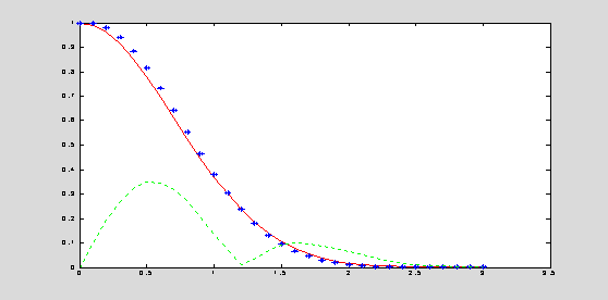
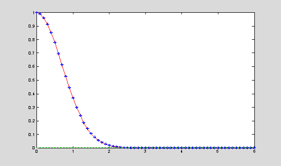
h = 0.1; y0 = 1; T = 3; n = T/h;

% differential equation: y' = -2*t*y, y(0) = 1

% exact solution: y(t) = exp(-t^2).

t(1) = 0; y(1) = y0; % the initial point in vectors (t,y)

for k = 1 : n

t(k+1) = t(k) + h;

y(k+1) = y(k) + h*(-2*t(k)*y(k));

end

yExact = exp(-t.^2); eLocal = 10*abs(y-yExact);

plot(t,yExact,'r',t,y,'*b',t,eLocal,':g');

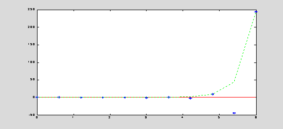
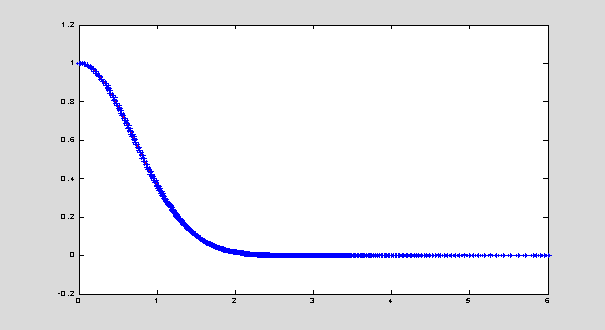
h = 0.6; y0 = 1; T = 6; n = T/h; t(1) = 0; y(1) = y0;

for k = 1 : n

t(k+1) = t(k) + h; y(k+1) = y(k) + h*(-2*t(k)*y(k));

end

yExact = exp(-t.^2); eLocal = abs(y-yExact);

plot(t,yExact,'r',t,y,'*b',t,eLocal,':g');

The forward Euler method is the simplest method for approximation the solution. It is of low accuracy and it may have stability problems for convergence of the iterative scheme.

· Backward Euler method:

Replace the derivative y'(t) at t = t_k by its backward difference approximation: (y_k-y_k-1)/h. Then, the differential equation becomes an implicit iterative scheme:

y_k+1 = y_k + h f(t_k+1,y_k+1)

The accuracy of the backward Euler method is the same as the accuracy of the forward Euler method, but the method is unconditionally stable. Since the right-hand-side is to be taken at the uknown value y_k+1, the method is implicit, i.e. a root finding algorithm has to be used to find the value of y_k+1 in the iterative scheme.

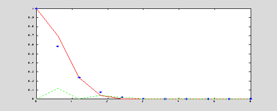
h = 0.6; y0 = 1; T = 6; n = T/h; t(1) = 0; y(1) = y0;

for k = 1 : n

t(k+1) = t(k) + h;

% solve the implicit equation: y(k+1) = y(k) + h*(-2*t(k+1)*y(k+1))

y(k+1) = y(k)/(1 + 2*h*t(k+1));

end, yExact = exp(-t.^2); eLocal = abs(y-yExact);

plot(t,yExact,'r',t,y,'*b',t,eLocal,':g');

· Improved Euler (Heun) method:

Rewrite the differential equation y' = f(t,y) as an implicit integral:

y(t_k+1) = y(t_k) + f(t,y(t)) dt

Apply the trapezoidal rule to the integral and derive the improved Euler method (also implicit):

y_k+1 = y_k + f(t_k,y_k) + f(t_k+1,y_k+1)

The improved Euler method has better accuracy than the forward or backward Euler methods, and it is also unconditionally stable. Since the right-hand-side is to be taken at the uknown value y_k+1, the method is implicit, i.e. a root finding algorithm has to be used to find the value of y_k+1 in the iterative scheme.

h = 0.1; y0 = 1; T = 6; n = T/h; t(1) = 0; y(1) = y0;

for k = 1 : n

t(k+1) = t(k) + h;

% solve the implicit equation:

% y(k+1) = y(k) + h*(-t(k)*y(k)-t(k+1)*y(k+1))

y(k+1) = y(k)*(1-h*t(k))/(1 + h*t(k+1));

end

yExact = exp(-t.^2); eLocal = abs(y-yExact);

plot(t,yExact,'r',t,y,'*b',t,eLocal,':g');

The idea of predictor-correctors can be used to represent the implicit improved Euler method as an explicit method. First, we predict the value y_n+1 at the time instance t_n+1 by the forward Euler method:

z_n+1 = y_n + h f(t_n,y_n)

where z_n+1 is the predicted value of y_n+1. Then, we correct this value with the improved Euler method:

y_k+1 = y_k + f(t_k,y_k) + f(t_k+1,z_k+1)

The pair of predictor-corrector formulas is explicit. It is known as the Heun method.

h = 0.1; y0 = 1; T = 6; n = T/h; t(1) = 0; y(1) = y0;

for k = 1 : n

t(k+1) = t(k) + h;

% prediction:

z = y(k) + h*(-2*t(k)*y(k));

% correction:

y(k+1) = y(k) + h*(-t(k)*y(k)-t(k+1)*z);

end

yExact = exp(-t.^2); eLocal = abs(y-yExact);

plot(t,yExact,'r',t,y,'*b',t,eLocal,':g');

More advanced methods for numerical solutions of differential equations:

· Runge-Kutta single-step methods

· Adams-Bashforth multi-step methods

MATLAB ODE solvers:

· ode23: Runge-Kutta solver of second and third order with variable step size

· ode45: Runge-Kutta solver of fourth and fifth order with variable step size

· ode113: Adams-Bashforth-Moulton solver of variable order from 1 to 13

· ode15s: stiff solver of variable order from 1 to 5 based on backward differentiation

· ode23s, ode23t, ode23tb: stiff solver of second and third order based on trapezoidal rule

[t,y] = ODEsolver(odefun,tspan,y0)

ODEsolver = name of the ODE solver

odeful = name of the ODE file (M-file function)

tspan = the initial and ending times [0, T] or the time interval partition [0 : h : T]

y0 = the initial value for differential equation

[t,y] = column vectors of the solution y = y(t) at the time points between 0 and T

function [y1] = ODEexample(t,y)

% ODE file (M-file function) for right-hand-side of the differential equation

% y1 if the derivative of the solution y = y(t) (the right-hand-side function)

y1 = -2*t*y;

y0 = 1; tspan = [0,6];

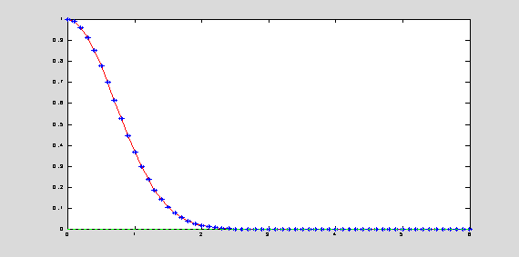
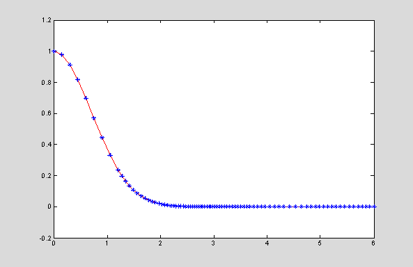
[t,y] = ode45(@ODEexample,tspan,y0);

t' % values of time instance where the solution is computed

yExact = exp(-t.^2); plot(t,yExact,'r',t,y,'*b');

Columns 1 through 11

0 0.1500 0.3000 0.4500 0.6000 0.7500 0.9000 1.0500 1.2000 1.2725 1.3449

Columns 12 through 22

1.4174 1.4898 1.5623 1.6347 1.7072 1.7796 1.8423 1.9050 1.9676 2.0303 2.0830

Columns 23 through 33

2.1357 2.1883 2.2410 2.2877 2.3345 2.3812 2.4279 2.4705 2.5131 2.5557 2.5983

Columns 34 through 44

2.6378 2.6773 2.7168 2.7563 2.7933 2.8303 2.8673 2.9043 2.9444 2.9846 3.0247

Columns 45 through 55

3.0648 3.1094 3.1539 3.1985 3.2431 3.2935 3.3439 3.3943 3.4448 3.5033 3.5619

Columns 56 through 66

3.6205 3.6790 3.7493 3.8196 3.8899 3.9602 4.0478 4.1355 4.2231 4.3108 4.4202

Columns 67 through 77

4.5295 4.6389 4.7483 4.8259 4.9036 4.9812 5.0589 5.1365 5.2142 5.2918 5.3695

Columns 78 through 85

5.4552 5.5410 5.6267 5.7124 5.7843 5.8562 5.9281 6.0000

options = odeset('optionname',optionvalue);

[t,y] = ODEsolver(odefun,tspan,y0,options);

RelTol - Relative error tolerance [ positive scalar {1e-3} ]

AbsTol - Absolute error tolerance [ positive scalar or vector {1e-6} ]

NormControl - Control error relative to norm of solution [ on | {off} ]

MaxStep - Upper bound on step size [ positive scalar ]

Additional parameters of the differential equation can be defined in the ODE M-file function and can be passed to the M-file function by additional input arguments of the ODE solver.

function [y1] = ODEexample(t,y,par)

% ODE file (M-file function) for right-hand-side of the differential equation

% y1 = the derivative of the solution y = y(t) (the right-hand-side function)

% par = additional parameter of the differential equation

y1 = -par*t*y;

y0 = 1; tspan = [0,6]; par = 2;

opt = odeset('AbsTol',10^(-10),'RelTol',10^(-8));

[t,y] = ode45(@ODEexample,tspan,y0,opt,par);

yExact = exp(-t.^2); plot(t,yExact,'r',t,y,'*b');

MATLAB BVP solver:

MATLAB has the following general boundary-value ODE solver:

[x,y,total] = bvp (alpha,beta,a,b,tol,n,q,g)

where y = y(x) is a solution of the second-order problem:

y'' = g(x,y,y'), a < x < b

with the boundary values: y(alpha) = a, y(beta) = b. Additional parameters are:

tol = upper bound on difference between numerical approximations;

n = number of interior solution points (m >= 1)

q = maximum number of iterations (q >= 1)

g = string containing name of a user-supplied M-file function in the form: y2 = function g (x,y,y1)

total= total number of iterations performed

[x,y]= column-vectors of the solution y = y(x) with (n+2) data points, including the two boundary points.