CHAPTER 4: MATHEMATICAL MODELING WITH MATLAB
Lecture 4.2: Summation rules
for numerical integration
Trapezoidal, Simpson and midpoint rules for
integrals:
Problem: Given a set of data points:
(x0,y0);
(x1,y1); (x2,y2); …(xn,yn)
Suppose
the data points represent a function y = f(x). Suppose also that
the data points are equally spaced with constant step size h = x1 -
x0. Find a numerical approximation for the integral, which
is the signed area under the curve y = f(x) between the end
points (x0,y0) and (xn,yn).
Example:
Linear
electrical circuits can be easily miniaturized if they do not include large and
bulky inductors. When a current I = I(t) is applied to the input
port of a simple resistor-capacitor one-port network, the voltage V = V(t) develops across the port
terminals. At the time instance t = T, the voltage output is
determined as a sum of the voltage drop across the resistor (which is R
I(T)) and of the voltage drop across the capacitor (which is V0
+  / C), where V0 is an initial
voltage. If the input current I(t) can be measured at different
times t = tk for k = 0,1,2,…,n, such
that t0 = 0 and tn = T, them
the integral is to be evaluated numerically from the given data set.
Solution:
The
function y = f(x) is either analytically defined or given in a
tabular form. The numerical integration is based on the use of numerical
interpolation y = Pn(x) fitted to the given data
points and analytical integration of the polynomial Pn(x). This
is a so-called Newton-Cotes integration algorithm. The most important
Newton-Cotes integration formulas are trapezoidal, Simpson and midpoint rules.
|
|
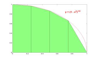
Trapezoidal rule: A
linear interpolation between the points (x0,y0)
and (x1,y1) approximates the area under
the curve y = f(x) by the area of the trapezoid: Trapezoidal
rule is popular in numerical integration as it is a simple method. Although
its accuracy is low, the accuracy can be controled by doubling the number of
elementary subintervals (trapezoids). |
|
|
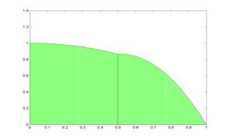
Simpson rule: A
quadratic interpolation between the points (x0,y0)
(x1,y1), and (x2,y2)
approximates the area under the curve y = f(x) by the
area under the interpolant: Simpson rule is popular because of high accuracy of
numerical integration compared to the trapezoidal rule. |
|
|
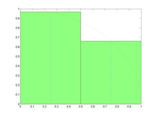
Mid-point rule: A
constant interpolation between the point (x1,y1),
centered in the interval between (x0,y0)
and (x2,y2), approximates the area under
the curve y = f(x) by the area of a rectangle centered at the
midpoint: Mid-point
rule is popular in numerical integration of functions with singularities at
the end of the interval. It has the same accuracy as the trapezoidal rule and
is often used in combination with the trapezoidal rule for computations of
integrals near singularities. |
h = 0.1; x0 = 0; x1 = x0+h; x2 = x0+2*h;
% the three data points are
taken on [0,1] with equal step size
y0 = sqrt(1-x0^2); y1 = sqrt(1-x1^2); y2 = sqrt(1-x2^2);
yIexact = quad('sqrt(1-x.^2)',x0,x2); % 'exact answer' is computed
by MATLAB
yItrap = h*(y0+y1+y1+y2)/2; % trapezoidal rule for two
subintervals with h
yIsimp = h*(y0+4*y1+y2)/3;
% Simpson rule for two subintervals with h
yImid = 2*h*y1; %
mid-point rule for two subintervals with h
fprintf('Exact = %6.6f\nTrapezoidal = %6.6f\nSimpson = %6.6f\nMid-point = %6.6f',yIexact,yItrap,yIsimp,yImid);
Exact = 0.198659
Trapezoidal = 0.198489
Simpson = 0.198658
Mid-point = 0.198997
Composite summation rules:
The
summation rules are extended to multiple intervals, when the function y =
f(x) is represented by (n+1) data points with constant
step size h. The composite rule is obtained by summating areas of
all n individual areas.
·
Composite trapezoidal rule:

![]() Itrapezoidal(f;x0,x1,…,xn)
=
Itrapezoidal(f;x0,x1,…,xn)
= ![]() ( y0 + 2 y1
+ 2 y2 + … + 2 yn-1 + yn )
( y0 + 2 y1
+ 2 y2 + … + 2 yn-1 + yn )
·
Composite Simpson rule:

![]() Isimpson(f;x0,x1,…,xn)
=
Isimpson(f;x0,x1,…,xn)
= ![]() ( y0 + 4 y1
+ 2 y2 + 4 y3 + 2 y4 + … + 2 yn-2 + 4 yn-1 +
yn )
( y0 + 4 y1
+ 2 y2 + 4 y3 + 2 y4 + … + 2 yn-2 + 4 yn-1 +
yn )
·
Composite mid-point rule:

![]() Imid-point(f;x0,x1,…,xn)
= 2h ( y1 + y3 +
… + yn-3 + yn-1 )
Imid-point(f;x0,x1,…,xn)
= 2h ( y1 + y3 +
… + yn-3 + yn-1 )
For
the composite Simpson and mid-point rules, the total interval between x ![]() [x0,xn] has to be divided into
even number of subintervals.
[x0,xn] has to be divided into
even number of subintervals.
Errors of numerical integration:
Numerical
integration is much more reliable process compared to numerical
differentiation. Rounding errors in computing sums in numerical integration are
always constant, which are independent neither of the integration rule nor from
the number of subintervals for summation. Truncation errors can be reduced with
the use of more accurate summation rules for numerical integration.
Consider
the equally spaced data points with constant step size: h = x2
– x1 = x1 – x0. The theory based on the Taylor expansion
method shows the following local truncation errors:
·
Trapezoidal rule:
![]() f(x)dx – Itrapezoidal(f;x0,x1 )
= -
f(x)dx – Itrapezoidal(f;x0,x1 )
= -![]() f''(x), x
f''(x), x ![]() [x0,x1]
[x0,x1]
The
truncation error of the trapezoidal rule is proportional to h3,
i.e. it has the order of O(h3). The error is also
proportional to the second derivative of the function f(x) at an
interior point x of the integration interval. Thus, the
trapezoidal rule is exact for a linear function f(x).
·
Simpson rule:
![]() f(x)dx – ISimpson(f;x0,x2 )
= -
f(x)dx – ISimpson(f;x0,x2 )
= - ![]() f''''(x), x
f''''(x), x ![]() [x0,x2]
[x0,x2]
The
truncation error of the Simpson rule is proportional to h5 rather
than h3, i.e. it has the order of O(h5).
The error is also proportional to the fourth derivative of the function f(x)
at an interior point x of the integration interval. The Simpson
rule is exact for polynomial functions f(x) of order m =
0,1,2,3.
·
Mid-point rule:
![]() f(x)dx – Imid-point(f;x0,x2 )
=
f(x)dx – Imid-point(f;x0,x2 )
= ![]() f''(x), x
f''(x), x ![]() [x0,x2]
[x0,x2]
The
truncation error of the mid-point rule is as bad as that of the trapezoidal
rule.
The global truncation error is computed for composite
integration rules when an interval between x![]() [x0,xn] is divided into n
partial subintervals. The global truncation error is obtained by
summation of local truncation errors and all local rounding errors:
[x0,xn] is divided into n
partial subintervals. The global truncation error is obtained by
summation of local truncation errors and all local rounding errors:
·
Composite trapezoidal rule:
etrapezoidal = |  - Itrapezoidal(f;x0,x1,…,xn)
| < M2
 ![]() (xn – x0) + eps (xn – x0),
(xn – x0) + eps (xn – x0),
where M2 = max | f''(x)|. The
global truncation error is proportional to the length of the integration
interval and is order of O(h2).
·
Composite Simpson rule:
eSimpson = |  - ISimpson(f;x0,x1,…,xn)
| < M4
 ![]() (xn – x0) + eps (xn – x0),
(xn – x0) + eps (xn – x0),
where M4 = max | f''''(x)|. The
global truncation error is proportional to the length of the integration
interval and is order of O(h4).
h = 0.1; k = 1;
while (h > 0.0000001)
x = 0 : h : 1; y =
sqrt(1.-x.^2); n = length(x)-1;
yIexact = pi/4; % exact
integral, 1/4 of area of a unit disk
yItrap =
h*(y(1)+2*sum(y(2:n))+y(n+1))/2; % composite trapezoidal rule
yIsimp =
h*(y(1)+4*sum(y(2:2:n))+2*sum(y(3:2:n-1))+y(n+1))/3;
yImid =
2*h*sum(y(2:2:n)); % composite
mid-point rule
eItrap(k) = abs(yItrap-yIexact); eIsimp(k) = abs(yIsimp-yIexact);
eImid(k) = abs(yImid-yIexact); hst(k) = h; h = h/2; k = k+1;
end,
plot(hst,eItrap,'g:',hst,eIsimp,'b--',hst,eImid,'r');
.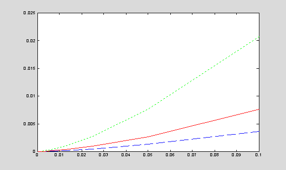
If
the step size h between two points becomes smaller, the
truncation error of the summation rule decreases. It decreases faster for
Simpson rule and slower for trapezoidal and mid-point rule. For example, if h
is halved, the global truncation error of the Simpson rule is
reduced by a factor of 16, while the global truncation errors of
the trapezoidal and mid-point rules are reduced only by a factor of 4.
Since
the rounding error is bounded by the integration interval multiplied by the
mashine precision eps, the error of numerical integration can be
reduced to that constant global number.
Example:
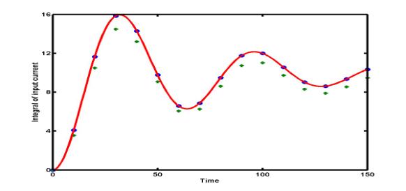
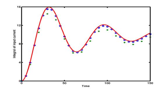
The
numerical approximations of the integral  , where I(t) is the current in a
resistor-capacitor network, are obtained with step size h = 10
(green pluses) and with step size h
= 5 (blue dots), versus the exact
integral (red solid curve). The composite trapezoidal rule's error
reduces with smaller step size h (blue dots are closer to the
exact red curve compared to the green pluses). The figure also shows that the
global truncation error for the integral grows with the length of the interval T.
MATLAB
numerical integration:
·
quad: evaluates
numerically the integral of a function by using adaptive Simpson quadrature
·
quadl: evaluates numerically the integral of a function by using adaptive
Lobatto quadrature
·
dblquad: evaluates the double integral of a function of two variables in a
rectangular domain
% The function for numerical integration
should be written as a MATLAB M-file
% The functon should
accept a vector argument X and return a vector result Y
function [Y] = integrand(X)
% this M-file sets up a
function y = f(x) = sqrt(1 + exp(x))
% which is the integrand
for the integral to be evaluated by function "quad"
Y = sqrt(1 + exp(X));
%
Compute the integral: I = int_0^2 sqrt(1 + exp(x)) dx
format long; I1 = quad(@integrand,0,2)
% the default tolerance is 10^(-6) for absolute error of numerical
integration
tolerance = 10^(-8); I2 = quad(@integrand,0,2,tolerance)
tolerance = 10^(-12); I3 = quad(@integrand,0,2,tolerance)
I4 = quadl(@integrand,0,2)
h = 0.0001; x = 0 : h : 2; y = feval(@integrand,x); n =
length(y)-1;
I5 = h*(y(1)+2*sum(y(2:n))+y(n+1))/2 % composite trapezoidal rule
I6 = h*(y(1)+4*sum(y(2:2:n))+2*sum(y(3:2:n-1))+y(n+1))/3 %
composite Simpson rule
I7 = 2*h*sum(y(2:2:n)) % composite mid-point rule
I2 = 4.00699422326706
I3 = 4.00699422325470
I4 = 4.00699422322700
I5 = 4.00699422402304
I6 = 4.00699422325470
I7 = 4.00699422171802
W1 =
quad('sin(pi*x.^2)',0,1), W2 = quad(inline('sin(pi*x.^2)'),0,1)
% standard MATLAB functions can be used for numerical integration as strings
W2 = 0.5049
Romberg integration for higher-order
Newton-Cotes integration formulas:
More
accurate integration formulas with smaller truncation error can be obtained by
interpolating several data points with higher-order interpolating polynomials.
For example, the third-order interpolating polynomial P3(x) between
four data points leads to the Simpson 3/8 rule:

![]() ISimpson 3/8(f;x0,x3)
=
ISimpson 3/8(f;x0,x3)
= ![]() ( y0 + 3y1 + 3y2 + y3 )
( y0 + 3y1 + 3y2 + y3 )
while
the fourth-order interpolating polynomial P4(x) between
five data points leads to the Booles rule:

![]() IBooles(f;x0,x4)
=
IBooles(f;x0,x4)
= ![]() ( 7 y0 + 32 y1 + 12 y2 + 32
y3 + 7 y4 )
( 7 y0 + 32 y1 + 12 y2 + 32
y3 + 7 y4 )
The
higher-order integration formulas can be recovered with the use of the Romberg
integration algorithm based on the Richardson extrapolation algorithm.
·
Recursive integration formulas:
The
composite trapezoidal rule has the global truncation error of order O(h2).
Denote the composite trapezoidal rule for the integral of f(x) between
[x0,xn] as R1(h).
Compute two numerical approximations of the integral with two step
sizes h and 2h:
![]() f(x) dx = R1(h) +
f(x) dx = R1(h) + ![]() h2 ;
h2 ; ![]() f(x) dx = R1(2h) + 4
f(x) dx = R1(2h) + 4![]() h4;
h4;
where
![]() is unknown
coefficient for the global truncation error. The number of trapezoids must be
even in order the numerical approximation with double step-size (2h)
could be computed. By cancelling the truncation error of order O(h2),
we define a new integration rule for the same integral:
is unknown
coefficient for the global truncation error. The number of trapezoids must be
even in order the numerical approximation with double step-size (2h)
could be computed. By cancelling the truncation error of order O(h2),
we define a new integration rule for the same integral:
![]() f(x) dx =
f(x) dx = ![]() = R2(h)
= R2(h)
The
new integration rule R2(h) for the same integral is
more accurate since the truncation error is of order O(h4). It
is in fact the composite Simpson's rule as it can be checked directly. If the
step size is sufficiently small, the composite Simpson's rule gives a much
better numerical approximation for the integral, compared to the composite
trapezoidal rule.
The
process can be continued to find a higher-order integration formulas Rm(h)
with the truncation error O(h2m). The recursive
formula for Romberg integration formulas:
Rm+1(h) =Rm(h)
+ ![]()
·
Numerical algorithm
There
are two modifications of the Romberg integration algorithm: with doubling the
step size h and with halving the step size. The first
modification is used when a limited number of data values is available. The
second modification is more preferable if the function y = f(x) is
available analytically and the data values (xk,yk) can
be computed for any step size h. In order to compute the
higher-order integration rules of the integral of f(x) between x0
![]() x
x ![]() xn up to the order m, the
number n must be matched with m as: n = 2m-1.
In this case, there are sufficient number of points to compute
integration rules of lower order with larger step sizes: h, 2h, 4h, 8h,
…, (m-1)h. The numerical approximations for the integrals can be
arranged in a table of recursive integration formulas starting with the
simplest approximation R1(h) (composite trapezoidal
rule):
xn up to the order m, the
number n must be matched with m as: n = 2m-1.
In this case, there are sufficient number of points to compute
integration rules of lower order with larger step sizes: h, 2h, 4h, 8h,
…, (m-1)h. The numerical approximations for the integrals can be
arranged in a table of recursive integration formulas starting with the
simplest approximation R1(h) (composite trapezoidal
rule):
|
step size |
R1 |
R2 |
R3 |
R4 |
R5 |
|
h |
R1(h) |
|
|
|
|
|
2h |
R1(2h) |
R2(h) |
|
|
|
|
4h |
R1(4h) |
R2(2h) |
R3(h) |
|
|
|
8h |
R1(8h) |
R2(4h) |
R3(2h) |
R4(h) |
|
|
16h |
R1(16h) |
R2(8h) |
R3(4h) |
R4(2h) |
R5(h) |
The
diagonal entries are values of higher-order integration rules for the integral
of f(x) between x0 ![]() x
x ![]() xn . The higher-order approximation Rk(h)
has the truncation error O(h2k). If h is
small, the truncation error rapidly decreases with larger k.
However, the rounding error is constant with larger value of k. As
a result, no further increase in accuracy of numerical integration can be
obtained after some number m
xn . The higher-order approximation Rk(h)
has the truncation error O(h2k). If h is
small, the truncation error rapidly decreases with larger k.
However, the rounding error is constant with larger value of k. As
a result, no further increase in accuracy of numerical integration can be
obtained after some number m ![]() M. The algorithm can be terminated when the relative
error falls below an error tolerance.
M. The algorithm can be terminated when the relative
error falls below an error tolerance.
Example:
The figure
below presents the numerical approximations R1(h) and
R2(h) for the integral of the current I(t) with
the step size h = 10. Blue circles are found by the composite
Simpson rule R2(h), green pluses are obtained by
composite trapezoidal rule R1(h), and the exact
integral of I(t) is shown by a red solid curve. The composite
Simpson rule R2(h) is clearly more accurate than the
composite trapezoidal rule R1(h).
