CHAPTER 4: MATHEMATICAL MODELING WITH MATLAB
Lecture 4.1: Finite
difference approximations for numerical derivatives
Forward, backward, and central differences
for derivatives:
Problem: Given a set of data points near the point (x0,y0):
…; (x-2,y-2);
(x-1,y-1); (x0,y0); (x1,y1);
(x2,y2); …
Suppose
the data values represent values of a function y = f(x). Find a
numerical approximation for derivatives f'(x0), f''(x0),
… of the function y = f(x) at the point (x0,y0).
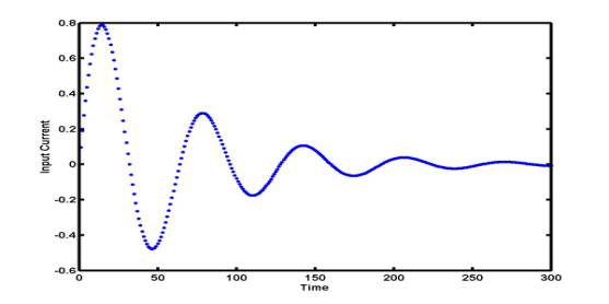
Example: Linear electrical circuits
consist of resistors, capacitors, inductors, and voltage and current sources.
In a simple resistor-inductor (RL) one-port network driven by a current source,
the voltage V = V(t) develops across the port terminals when a
current I = I(t) is applied to the input port, The voltage output
V(t) can be determined as a sum of the voltage drop across the
resistor R I(t) and of the voltage drop across the inductor L
I'(t). The derivative I'(t) is to be found from the input
current I(t) measured at different time instances:
Solution:
The first
derivative f'(x0) of the function y = f(x)
at the point (x0,y0) can be
approximated by the slope of the secant line that passes through two points
(linear piecewise interpolation). Depending on whether the points are taken to
the right of the point (x0,y0) (future data), to the left of the point (x0,y0)
(past data), or to both sides, the slope of the secant line is called the
forward, backward or central difference approximations.
|
|
Forward difference approximation: The secant line passes the points (x0,y0)
and (x1,y1). f'(x0) Forward
differences are useful in solving initial-value problems for differential
equations by single-step predictor-corrector methods (such as Euler methods).
Given the values f'(x0) and f(x0),
the forward difference approximates the value f(x1). |
|
|
Backward difference approximation: The secant line passes the points (x-1,y-1)
and (x0,y0).
f'(x0) Backward differences are useful for approximating the
derivatives if the data values are available in the past but not in the
future (such as secant methods for root finding and control problems). Given
the values f(x-1) and f(x0),
the backward difference approximates the value f(x1),
if it depends on f'(x0). |
|
|
Central difference approximation: The secant line passes the points (x-1,y-1)
and (x1,y1). f'(x0) Central
differences are useful in solving boundary-value problems for differential
equations by finite difference methods. Approximating values of f'(x0)
that occurs in differential equations or boundary conditions, the central
difference relates unknown values f(x-1) and f(x1) by an
linear algebraic equation. |
h = 0.1; x0 = 1; x_1 =
x0-h; x1 = x0 + h;
% the three data points are located at equal distance h (the step
size)
y0 = exp(10*x0); y_1 = exp(10*x_1); y1 = exp(10*x1); yDexact =
10*exp(10*x0);
yDforward = (y1-y0)/h; % simple form of forward difference for
equally spaced grid
yDbackward = (y0-y_1)/h; %
simple form of backward difference
yDcentral = (y1-y_1)/(2*h);
% simple form of central difference
fprintf('Exact = %6.2f\nForward = %6.2f\nBackward = %6.2f\nCentral = %6.2f',yDexact,yDforward,yDbackward,yDcentral);
Forward = 378476.76
Backward = 139233.82
Central = 258855.29
Errors of numerical differentiation:
Numerical
differentiation is inherently ill-conditioned process. Two factors determine
errors induced when the derivative f'(x0) is replaced
by a difference approximations: truncation and rounding errors.
Consider
the equally spaced data points with constant step size: h = x1
– x0 = x0 – x-1. The theory based on the Taylor expansion
method shows the following truncation errors:
·
Forward difference approximation:
f'(x0) – Dforward(f,x0)
= -![]() f''(x), x
f''(x), x ![]() [x0,x1]
[x0,x1]
The
truncation error of the forward difference approximation is proportional to h,
i.e. it has the order of O(h). The error is also proportional to
the second derivative of the function f(x) at an interior point x
of the forward difference interval.
·
Backward difference approximation:
f'(x0) – Dbackward(f,x0)
= ![]() f''(x), x
f''(x), x ![]() [x-1,x0]
[x-1,x0]
The
truncation error of the backward difference approximation is as bad as that of
the forward difference approximation. It also has the order of O(h)
and is also proportional to the second derivative of the function f(x)
at an interior point x of the backward difference interval.
·
Central difference approximation:
f'(x0) – Dcentral(f,x0)
= -![]() f'''(x), x
f'''(x), x ![]() [x-1,x1]
[x-1,x1]
The
truncation error of the central difference approximation is proportional to h2
rather than h, i.e. it has the order of O(h2).
The error is also proportional to the third derivative of the function f(x)
at an interior point x of the central difference interval. The
central difference approximation is an average of the forward and backward
differences. It produces a much more accurate approximation of the derivative
at a given small value of h, compared to the forward and backward
differences. If the data values are available both to the right and to the left
of the point (x0,y0), the use of the
central difference approximation is the most preferable.
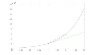
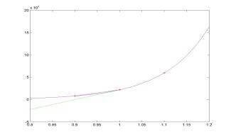
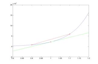
x0 = 1; x_1 = x0-h; x1 = x0+h;
y0 = exp(10*x0); y_1 = exp(10*x_1); y1 = exp(10*x1); yDe =
10*exp(10*x0);
yDf = (y1-y0)./h; yDb = (y0-y_1)./h; yDc = (y1-y_1)./(2*h);
eDf = abs(yDf-yDe); eDb = abs(yDb-yDe); eDc = abs(yDc-yDe);
loglog(h,eDf,'g:',h,eDb,'b--',h,eDc,'r');
If
the step size h between two points becomes smaller, the truncation
error of the difference approximation decreases. It decreases faster for
central difference approximations and slower for forward and backward
difference approximations. For example, if h is reduced by a
factor of 10, the truncation error of the central difference
approximation is reduced by a factor of 100, while the truncation
errors of the forward and backward differences are reduced only by a factor of 10.
When
h becomes too small, the difference approximations are taken for
almost equal values of f(x) at the two points. Any rounding error
of computations of f(x) is magnified by a factor of 1/h. As
a result, the rounding error grows with h for very small values
of h. An optimal step size h = hopt can
be computed from minimization of the sum of truncation and rounding errors:
·
Forward difference approximation:
eforward = | f'(x0)
– Dforward(f,x0)| <
M2 ![]() + 2
+ 2 ![]() ,
,
where
M2 = max | f''(x)|. The minimum of error occurs for h
= hopt =2![]() , when eforward = 2
, when eforward = 2![]() .
.
·
Central difference approximation:
ecentral = | f'(x0)
– Dcentral(f,x0)| < M3 ![]() + 2
+ 2 ![]() ,
,
where
M3 = max | f'''(x)|. The minimum of error occurs for h
= hopt =![]() , when eforward = 3
, when eforward = 3![]() .
.
M3 = 1000*exp(10*(x0+0.1));
hoptForward = 2*(eps/M2)^(1/2)
hoptCentral = (6*eps/M3)^(1/3)
eoptForward = 2*(eps*M2)^(1/2)
eoptCentral = 3*(eps^2*M3/6)^(1/3)
hoptCentral = 2.8127e-008
eoptForward = 7.2924e-005
eoptCentral = 2.3683e-008
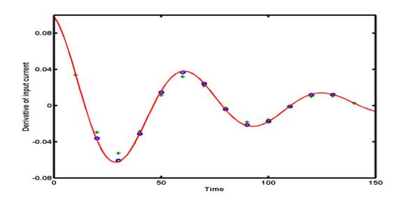
Example: Two central difference
approximations are applied to compute the derivative of the current I'(t):
green pluses are for h = 10 and blue dots are for h = 5.
The exact derivative I'(t) is shown by red solid curve.
Newton forward difference interpolation:
Problem: Given a set of (n+1) data points:
(x1,y1);
(x2,y2); …; (xn,yn); (xn+1,yn+1)
Find
a Newton polynomial of degree n, y = Pn(x), that passes through all (n+1) data
points. The Newton polynomial is a discrete Taylor polynomial of the form:
y = Pn(x) = c0
+ c1 (x-x1) + c2(x-x1)(x-x2)
+ cn (x – x1)(x – x2)…(x-xn)
where the coefficients cj are
constructed from diagonal divided differences.
Comparison:
Lagrange
polynomial interpolation is convenient when the same grid points [x1,x2,…,xn+1]
are
repeatevely used in several applications. The data values can be stored in
computer memory to reduce a number. The Lagrange interpolation is not useful
however when additional data points are added or removed to improve the
appearance of the interpolating curve. The data set has to be completely
recomputed every time when the data points are added or removed. The Newton
polynomial interpolation is more convenient for adding and deleting additional
data points. It is also more convenient for an algorithmic use of the Horner's
nested multiplication. Of course, the Newton interpolating polynomials
coincides with the Vandermond and Lagrange interpolating polynomials for a
given data set, since the interpolating polynomial y = Pn(x) of
order n connecting (n+1) data points are unique.
The difference between Vandermonde, Lagrange, and Newton interpolating
polynomials lies only in computational aspects.
Solution:
The
coefficients cj are to be found from the conditions: Pn(xk)
= yk that results in a linear system:
Ac
= y. The
Gauss elimination algorithm or induction methods can be used to prove that cj
= dj,j, where dj,j are diagonal
entries in the table of forward divided differences:
|
grid points |
data values |
first differences |
second differences |
third differences |
fourth differences |
|
x1 |
y1 |
|
|
|
|
|
x2 |
y2 |
f[x1,x2] |
|
|
|
|
x3 |
y3 |
f[x2,x3] |
f[x1,x2,x3] |
|
|
|
x4 |
y4 |
f[x3,x4] |
f[x2,x3,x4] |
f[x1,x2,x3,x4] |
|
|
x5 |
y5 |
f[x4,x5] |
f[x3,x4,x5] |
f[x2,x3,x4,x5] |
f[x1,x2,x3,x4,x5] |
Zero
divided differences f[xk] are simply the values of the function y =
f(x) at the point (xk,yk). First
divided differences f[xk,xk+1] are forward
difference approximation for derivatives of the function y = f(x)
at (xk,yk):
f[xk,xk+1]
= ![]()
Second,
third, and higher-order forward divided difference are constructed by using the
recursive rule:
f[xk,xk+1,…,xk+m]
= ![]()
With
the use of divided differences cj-1 = f[x1,x2,…,xj],
the Newton interpolating polynomial y = Pn(x) has
the explicit representation:
Pn(x) = ![]() f[x1,x2,…,xj]
f[x1,x2,…,xj] 
% example of explicit computation of
coefficients of Newton polynomials
x = [ -1,-0.75,-0.5,-0.25,-0]; n = length(x)-1;
y = [ -14.58,-6.15,-1.82,-0.23,-0.00];
A = ones(n+1,1); % the coefficient matrix for
linear system Ac = y
for j = 1 : n
A = [ A,
A(:,j).*(x'-x(j))];
end
A, c = A\(y'); c = c'
1.0000 0.2500 0 0 0
1.0000 0.5000
0.1250 0 0
1.0000 0.7500
0.3750 0.0938 0
1.0000 1.0000
0.7500 0.3750 0.0938
c = -14.5800 33.7200 -32.8000 14.5067 0.2133
function [yi,c]
= NewtonInter(x,y,xi)
% Newton interpolation algorithm
% x,y - row-vectors of (n+1) data values (x,y)
% xi - a row-vector of x-values, where interpolation is to be
found
% yi - a row-vector of interpolated y-values
% c - coefficients of Newton interpolating polynomial
n = length(x) - 1; % the degree of interpolation polynomial
ni = length(xi); % the number of x-values, where interpolation is
to be found
D = zeros(n+1,n+1); % the matrix for Newton divided differences
D(:,1) = y'; % zero-order divided differences
for k = 1 : n
D(k+1:n+1,k+1) =
(D(k+1:n+1,k)-D(k:n,k))./(x(k+1:n+1)-x(1:n-k+1))';
end
c = diag(D);
% computation of values of the Newton interpolating polynomial at
values of xi
% the algorithm uses the Horner's rule for polynomial evaluation
yi = c(n+1)*ones(1,ni); % initialization of the vector yi as the
coefficient of the highest degree
for k = 1 : n
yi =
c(n+1-k)+yi.*(xi-x(n+1-k)); % nested multiplication
end
x = [
-1,-0.75,-0.5,-0.25,-0]; y = [ -14.58,-6.15,-1.82,-0.23,-0.00];
xInt = -1 : 0.01 : 0;
[yInt,c] = NewtonInter(x,y,xInt);
c = c', plot(xInt,yInt,'g',x,y,'b*');
c = -14.5800 33.7200
-32.8000 14.5067 0.2133
MATLAB
finite differences:
Let
the data points x1,x2,…,xn,xn+1
be equally spaced with constant step size h = x2 – x1.
Then, the divided differences can be rewritten as:
f[xk,xk+1,…,xk+m]
= ![]() ,
,
where
![]() is the m-th forward
difference of a function y = f(x) at the point (xk,yk).
is the m-th forward
difference of a function y = f(x) at the point (xk,yk).
![]() = y1 – y0
= y1 – y0
![]() = y2 – 2 y1
+ y0
= y2 – 2 y1
+ y0
![]() = y3 –3 y2
+ 3 y1 – y0
= y3 –3 y2
+ 3 y1 – y0
![]() = y4 – 4 y3
+ 6 y2 -4 y1 – y0
= y4 – 4 y3
+ 6 y2 -4 y1 – y0
![]() = y5 – 5 y4
+ 10 y3 – 10 y2 + 5 y1 – y0
= y5 – 5 y4
+ 10 y3 – 10 y2 + 5 y1 – y0
Derivatives
of the interpolation polynomials y = Pn(x) approximate
derivatives of the function y = f(x). Matching the n-th derivative
of the polynomial y = Pn(x) with f(n)(x0),
we find the forward difference approximation for higher-order
derivatives:
f(n)(x0)
![]()
![]()
·
diff(y): computes first-order forward difference for a given vector y
·
diff(y,n): computes n-th order forward difference for a given vector
y
·
gradient(u): computes horizontal and vertical forward differences for a given matrix
to approximate the x- and y-derivatives of u(x,y):
grad(u) = [ux,uy]
·
del2(u): computes a discrete Laplacian for a given matrix u: ![]() u = uxx + uyy
u = uxx + uyy
n = 50; x =
linspace(0,2*pi,n); h = x(2)-x(1); y = sin(x); % function
y1 = diff(y)/h; y2 = diff(y,2)/h^2; y1ex = cos(x); y2ex =
-sin(x);% derivatives
plot(x(1:n-1),y1,'b',x,y1ex,':r',x(1:n-2),y2,'g',x,y2ex,':r');
Hierarchies of higher-order difference
approximations:
Newton
interpolating polynomials and divided difference tables can be constructed for
backward differences, since the order of data points x1,x2,…,xn,xn+1
is arbitrary. By arranging for data points in descenting order, the Newton
polynomial represents the backward differences. It is trickier to construct
tables for central differences. Since central differences are the most accurate
approximations, special algorithms are designed to automate derivation of
coefficients of central difference approximations for higher-order derivatives.
·
hierarchy of forward differences:
Let
the data points are equally spaced with constant step size h. Fix
a point (x0,y0) and present a forward
difference approximation for the n-th derivative as the inner
product multiplication:
f(n)(x0)
![]()
![]() Dn*y
Dn*y
where
y = [ y0,y1,y2, …]
n = 100; A = diag(ones(n-1,1),1)-diag(ones(n,1));
m = 8; B = A;
for k = 1 : m-1
D(k,:) = B(1,1:m);
B = B*A;
end
D = D
1 -2
1 0 0 0 0
0
-1 3
-3 1 0
0 0 0
1 -4
6 -4 1 0 0
0
-1 5
-10 10 -5
1 0 0
1 -6
15 -20 15
-6 1 0
-1 7 -21 35 -35 21 -7 1
·
hierarchy of central differences
Let
the data points are equally spaced with constant step size h. Fix
a point (x0,y0) and present a central
difference approximation for the n-th derivative as the inner
product multiplication:
f(2m-1)(x0)
![]()
![]() D2m-1*y;
f(2m)(x0)
D2m-1*y;
f(2m)(x0) ![]()
![]() D2m*y
D2m*y
where
y = [ …,y-2,y-1,y0,y1,y2,
…]
n = 100; A = diag(ones(n-1,1),1)-diag(ones(n-1,1),-1);
A2 = diag(ones(n-1,1),1)+diag(ones(n-1,1),-1)-2*diag(ones(n,1));
m = 4; B = A; C = A2; k = 1;
while (k < (2*m-2) )
D(k,:) = B(m,1:2*m-1);
D(k+1,:) = C(m,1:2*m-1);
B = B*A2; C = C*A2;
k = k+2;
end
D = D
0 0
1 -2 1 0 0
0 -1
2 0 -2 1 0
0 1
-4 6 -4
1 0
-1 4
-5 0 5
-4 1
1 -6 15 -20 15 -6 1
Richardson extrapolation for higher-order
differences:
Recursive
difference formulas for derivatives can be obtained by canceling the truncation
error at each order of numerical approximation. This method is called the
Richardson extrapolation. It can be used only if the data values are equally
spaced with constant step size h.
·
Recursive forward differences:
The
hierarchy of forward differences for first and higher-order derivatives has the
truncation error of order O(h). Denote the forward difference
approximation for a derivative f(n)(x0) as
D1(h). Compute the approximation with two step sizes h
and 2h:
f(n)(x0)
= D1(h) + ![]() h; f(n)(x0)
= D1(2h) + 2
h; f(n)(x0)
= D1(2h) + 2![]() h
h
where
![]() is unknown
coefficient for the truncation error. By cancelling the truncation error of
order O(h), we define a new forward difference approximation for
the same derivative:
is unknown
coefficient for the truncation error. By cancelling the truncation error of
order O(h), we define a new forward difference approximation for
the same derivative:
f(n)(x0)
= 2D1(h) – D1(2h) = D2(h)
The
new forward difference approximation D2(h) for the
same derivative is more accurate since the truncation error is of order O(h2).
- First-order derivative f'(x0):
The
first-order approximation D1(h) is a two-point divided
difference, while the second-order approximation D2(h)
is a three-point divided difference:
D1(h) = ![]() , D2(h) =
, D2(h) = ![]()
- Second-order derivative f''(x0):
The
first-order approximation D1(h) is a three-point
divided difference, while the second-order approximation D2(h)
is a four-point divided difference:
D1(h) = ![]() , D2(h) =
, D2(h) = ![]()
The
process can be continued to find a higher-order forward-difference
approximation Dm(h) with the truncation error O(hm).
The recursive formula for Richardson forward difference extrapolation:
Dm+1(h) =Dm(h)
+ ![]()
·
Recursive central differences:
The
hierarchy of central differences for first and higher-order derivatives has the
truncation error of order O(h2). Denote the central
difference approximation for a derivative f(n)(x0) as
D1(h). Compute the approximation with two step sizes h
and 2h:
f(n)(x0)
= D1(h) + ![]() h2; f(n)(x0)
= D1(2h) + 4
h2; f(n)(x0)
= D1(2h) + 4![]() h2
h2
where
![]() is unknown
coefficient for the truncation error. By cancelling the truncation error of
order O(h2), we define a new central difference
approximation for the same derivative:
is unknown
coefficient for the truncation error. By cancelling the truncation error of
order O(h2), we define a new central difference
approximation for the same derivative:
f(n)(x0)
= ![]()
The
new central difference approximation D2(h) for the
same derivative is more accurate since the truncation error is of order O(h4).
- First-order derivative f'(x0):
The
first-order approximation D1(h) is a three-point
divided difference, while the second-order approximation D2(h)
is a five-point divided difference:
D1(h) = ![]() , D2(h) =
, D2(h) =
![]()
- Second-order derivative f''(x0):
The
first-order approximation D1(h) is a three-point
divided difference, while the second-order approximation D2(h)
is a five-point divided difference:
D1(h) = ![]() , D2(h) =
, D2(h) =
![]()
The
process can be continued to find a higher-order central-difference
approximation Dm(h) with the truncation error O(h2m).
The recursive formula for Richardson forward difference extrapolation:
Dm+1(h) =Dm(h)
+ ![]()
·
Numerical algorithm
In
order to compute the central difference approximation of a derivative f(n)(x0)
up to order m, central difference approximations of lower
order are to be computed with larger step sizes: h, 2h, 4h, 8h, …,
(m-1)h.
These
approximations can be arranged in a table of recursive derivatives:
|
step size |
D1 |
D2 |
D3 |
D4 |
D5 |
|
h |
D1(h) |
|
|
|
|
|
2h |
D1(2h) |
D2(h) |
|
|
|
|
4h |
D1(4h) |
D2(2h) |
D3(h) |
|
|
|
8h |
D1(8h) |
D2(4h) |
D3(2h) |
D4(h) |
|
|
16h |
D1(16h) |
D2(8h) |
D3(4h) |
D4(2h) |
D5(h) |
The
diagonal entries are values of higher-order central difference approximations
for the derivative f(n)(x0)
where
x0 is the central point surrounded by the points x
= x0 - 2k-1h and x = x0 + 2k-1h
for k = 1,2,…,m.
The
higher-order approximation Dk(h) has the truncation
error O(h2k). If h is small, the
truncation error rapidly decreases with larger k. However, the
rounding error grows with larger value of k. An optimal order m
exists at the minimum of the sum of the truncation and rounding errors.
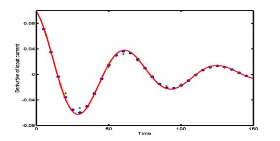
Example:
The figure
below presents the central difference approximations D1(h) and
D2(h) for the derivative of the current I(t) with
the step size h = 10. Blue circles are found by five-point
central differences D2(h), green pluses are obtained
by three-point central differences D1(h), and the
exact derivative I'(t) is shown by a red solid curve. Five-point
difference approximation D2(h) is clearly more
accurate than the three-point difference D1(h).