CHAPTER 3: NUMERICAL ALGORITHMS WITH MATLAB
Lecture 3.5: Two-dimensional
interpolation and errors of polynomial interpolation
Two-dimensional interpolation:
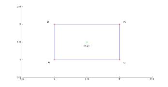
Problem: Given four data points on a
rectangular grid in space of three dimensions:
(x1,y1,z1);
(x2,y2,z2); (x3,y3,z3);
(x4,y4,z4)
Find
the value of z at the interior point of the rectangle.
Example:
Four data
points are:
|
|
A |
B |
C |
D |
|
|
x |
1 |
1 |
2 |
2 |
|
|
y |
1 |
2 |
1 |
2 |
|
|
z |
5 |
8 |
7 |
10 |
The
data points are evaluated at the plane: z = 2x + 3y. Find an
interpolation of the function at the interior (center) point (x,y).
·
interpl2: computes interpolation of values of z at the points
(x,y) from a set of data values (xi,yi,zi).
x = [ 1,2]; y
= [1,2]; [X,Y] = meshgrid(x,y)
z = 2*X+3*Y % data values at the vertex points of (x,y)
xInt = 1.5; yInt = 1.5; zInt = interp2(x,y,z,xInt,yInt)
zExact = 2*xInt + 3*yInt % exact value at the center point
1 2
Y = 1 1
2 2
z = 5 7
8 10
zInt = 7.5000
zExact = 7.5000
x = [1,2,3]; y = [1,2,3]; [X,Y] =
meshgrid(x,y); z = 2*X+3*Y;
zInt = interp2(x,y,z,xInt,yInt,'linear') % bilinear interpolation
zInt = interp2(x,y,z,xInt,yInt,'spline') % bicubic spline
interpolation
zInt = interp2(x,y,z,xInt,yInt,'cubic') % bicubic Hermite interpolation
zInt = 7.5000
zInt = 7.5000
·
datagrid: fits a surface of the form to the data in the nonuniformly-spaced
vectors (X,Y,Z)
o
methods
of interpolations in "datagrid" are different from those in "interpl2"
o
methods
of interpolations in "datagrid" are based on a Delaunay
triangulation of the data.
[x,y,z] = peaks(10); [xi,yi] = meshgrid(-3:.1:3,-3:.1:3);
zi = interp2(x,y,z,xi,yi,'cubic'); mesh(xi,yi,zi)
|
|
|
Solution
of the problem:
1D interpolation along [A,B]: z[A,B] = zA
![]() + zB
+ zB ![]()
1D interpolation along [C,D]: z[C,D] = zC
![]() + zD
+ zD ![]()
1D interpolation along [(A,B),(C,D)]: z = z[A,B] ![]() + z[C,D]
+ z[C,D]![]()
x = [1,2]; y
= [1,2]; z = [ 5,7;8,10]; xInt = 1.5; yInt = 1.5;
zAB =
z(1,1)*(yInt-y(2))/(y(1)-y(2))+z(2,1)*(yInt-y(1))/(y(2)-y(1));
zCD =
z(1,2)*(yInt-y(2))/(y(1)-y(2))+z(2,2)*(yInt-y(1))/(y(2)-y(1));
zInt = zAB*(xInt-x(2))/(x(1)-x(2))+zCD*(xInt-x(1))/(x(2)-x(1))
Errors
of polynomial interpolation:
The
truncation error between the function y = f(x) and the
interpolating polynomial y = Pn(x) between (n+1) data points is
proportional to the remainder polynomial of the (n+1)-th order:
| f(x) – Pn(x) | ![]()
![]() |(x-x1)(x-x2)…(x-xn)(x-xn+1)|, Mn+1 =
|(x-x1)(x-x2)…(x-xn)(x-xn+1)|, Mn+1 = ![]() | f(n+1)(x)|
| f(n+1)(x)|
If
the data points are equally spaced with constant step size h,
then the local error of the polynomial interpolation en(x) = |
f(x) – Pn(x) | is bounded as:
| f(x) – Pn(x) | ![]() hn+1
hn+1
The
error decreases if the step size h becomes smaller with a fixed
number of data points (n+1). If the interpolation interval is
fixed, the number of data points (n+1) grows with smaller step
size. In this case, the truncation error decreases with larger values of n.
However, the rounding error increases with larger values of n.
As a result, the polynomial interpolation becomes worse with larger number of
points after some optimal number n = nopt!
x =
linspace(0,pi,7); y = sin(x);
% given function with 7
equispaced data points
c = polyfit(x,y,6); xInt = linspace(0,pi,100); yInt =
polyval(c,xInt);
% polynomial
interpolation on a tense grid
yExact = sin(xInt); eLocal = abs(yExact-yInt);
% exact values and
local error e(x) of the polynomial interpolation
plot(xInt,eLocal)
The
local error en(x) vanishes at the data points x
= x1,x2,…,xn,xn+1. The
local error has local maxima at the centers between the two adjacent points.
The local error is larger at the ends of the interpolation interval. The local
error is smaller in the middle of the interpolation interval. These properties
are typical for polynomial interpolation with equally spaced data points. They
are explained by the behaviour of the remainder polynomial of the (n+1)-th
order.
% error of polynomial interpolation with
smaller h and fixed n
m = 10;
for k = 1 : m
x = linspace(0,pi*(m-k+1)/m,7); y = sin(x);
h(k) = x(2)-x(1); % step size of the data points
c = polyfit(x,y,6);
xInt = linspace(0,pi*(m-k+1)/m,100); yInt = polyval(c,xInt);
yExact = sin(xInt); eLocal
= abs(yExact-yInt);
eGlobal(k) =
norm(eLocal,2); % global error as the total mean square error
end
plot(h,eGlobal,'*')
a = polyfit(log(h),log(eGlobal),1);
% Checking the theory:
eGlobal = c h^(n+1)
% In log-log scale:
log(eGlobal) = (n+1) log(h) + log(c)
% The first coefficient of
the linear regression must be approximately 7
power = a(1)
% error of
polynomial interpolation with smaller h and fixed interval [0,pi]
m = 60;
for n = 1 : m
x = linspace(0,pi,n+1); y = sin(x);
h(n) = x(2)-x(1); % step size of the data points
c = polyfit(x,y,n);
xInt = linspace(0,pi,100); yInt = polyval(c,xInt);
yExact = sin(xInt); eLocal
= abs(yExact-yInt);
eGlobal(n) =
norm(eLocal,2); % global error as the total mean square error
end
semilogy(eGlobal,'*');
% the optimal number n = nOpt occurs where the total of
% truncation error and rounding error reaches the minimal value
% The optimal number is approximately nOpt = 18
% The polynomial interpolation becomes worse with larger values of
n.
% error of trigonometric interpolation with smaller h and fixed
interval [-1,1]
Nmax = 60;
for m = 1 : Nmax
x = linspace(-1,1,2*m+1); y
= 1./(1 + 25*x.^2);
n = 2*m; L = 2; xx =
[x(m+1:n),x(1:m)]'; yy = [y(m+1:n),y(1:m)]';
for j = 0 : m
a(j+1) = 2*yy'*cos(2*pi*j*xx/L)/n;
b(j+1) = 2*yy'*sin(2*pi*j*xx/L)/n;
end
xInt = linspace(-1,1,201);
yInt = 0.5*a(1)*ones(1,length(xInt));
for j = 1 : (m-1)
yInt = yInt + a(1+j)*cos(2*pi*j*xInt/L) +
b(1+j)*sin(2*pi*j*xInt/L);
end
yInt = yInt +
a(m+1)*cos(2*pi*m*xInt/L);
yExact =
1./(1 + 25*xInt.^2); eLocal = abs(yExact-yInt);
eGlobal(n)
= norm(eLocal,2); % global error as the total mean square error
end
semilogy(eGlobal,'*');
% The error of trigonometric interpolation decreases with larger n