CHAPTER 3: NUMERICAL ALGORITHMS WITH MATLAB
Lecture 3.3: Piecewise
polynomial interpolation
Piecewise interpolation:
Problem: Given a set of (n+1) data points:
(x1,y1);
(x2,y2); …; (xn,yn); (xn+1,yn+1)
Find
a smooth function y = S(x) that connects the given set of (n+1)
data points. The function y = S(x) consists of low-order
polynomials y = Sj(x) that connect two consecutive
data points: (xj,yj) and (xj+1,yj+1).
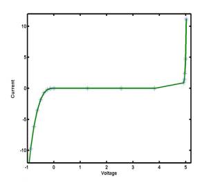
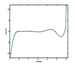
Example: Given a set of seven data points for a
voltage-current characteristic of a zener diode
|
Voltage |
-1.00 |
0.00 |
1.27 |
2.55 |
3.82 |
4.92 |
5.02 |
|
Current |
-14.58 |
0.00 |
0.00 |
0.00 |
0.00 |
0.88 |
11.17 |
If
the seven points are connected by a polynomial y = P6(x) of
order 6, the continuous polynomial interpolation is not good
because of large swings of the interpolating polynomial between the data
points:
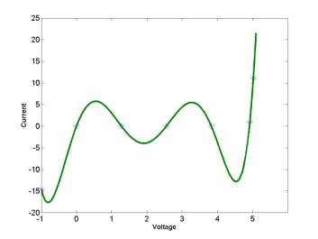
The
polynomial y = P6(x) of order 6 may have five extremal
points (maxima and minima). Indeed, all five extrema are seen on the picture
above. This is called the polynomial wiggle. If n is
large, interpolating polynomials show large errors and are rarely used for
graphical visualization of curves. Instead, the piecewise interpolation made of
polynomials of lower order is used to represent a sufficiently smooth curve y
= S(x):
|
|
|
·
interp1: applies a piecewise interpolation between given set of data points
x = [
-1,-.866,-.5,0,0.5,0.866,1,1.0402,1.15,1.3,1.54,1.828,2.1736,2.5883,3.086];
y = [
0,-0.25,-0.433,-0.5,-0.433,-0.25,0,0.15,0.2598,0.3,0.3,0.3,0.3,0.3,0.3];
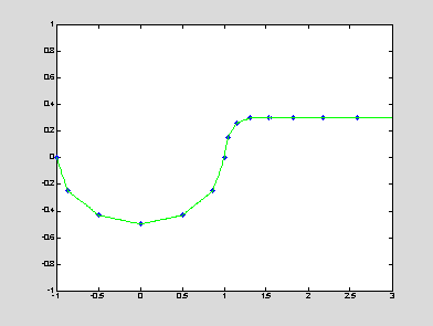
xInt = -1 : 0.01 : 3; yInt = interp1(x,y,xInt); % default linear
interpolation
plot(x,y,'b*',xInt,yInt,'g'); axis([-1,3,-1,1]);
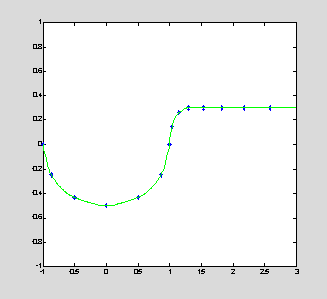
yInt = interp1(x,y,xInt,'spline'); % piecewise
cubic spline interpolation
plot(x,y,'b*',xInt,yInt,'g'); axis([-1,3,-1,1]);
yInt = interp1(x,y,xInt,'cubic'); % piecewise cubic Hermite
interpolation
plot(x,y,'b*',xInt,yInt,'g'); axis([-1,3,-1,1]);
|
|
|

· ppval: computes values of the cubic spline and Hermite interpolants in their pp-representations
% computes the value of y
at x = -0.25 of the cubic spline interpolant
y2 = ppval(pchip(x,y),-0.25)
% computes the value of y at x = -0.25 of the cubic Hermite interpolant
y2 = -0.4801
· unmkpp: extracts breaks, coefficients, number of pieces, and order from the cubic spline and Hermite interpolants in their pp-representations
[P,R,n,m] = unmkpp(spline(x,y))
% P is the vector of x
containing break points (length: n+1)
% R is the matrix of
coefficients of cubic spline interpolants (size: n-by-m)
% n – number of pieces of
the interpolants (length(x)-1)
% m – number of coefficients in each piece (order of the
polynomial + 1)
% Example: n = 3 and m = 4
% Sj(x) = aj + bj*(x-xj) +
cj*(x-xj)^2 + dj*(x-xj)^3 – piece between [xj,xj+1]
% aj = R(:,4); bj = R(:,3); cj = R(:,2); dj = R(:,1);
R = 8.6251
-41.7147 43.9131 5.1765
8.6251 -15.8394 -13.6409
16.0000
8.6251 10.0360 -19.4443
-4.8552
n = 3
m = 4
[P,R,n,m] = unmkpp(pchip(x,y))
R = 5.0158
-20.8552 26.6629 5.1765
40.2008 -61.0560 0
16.0000
0.0567 0.6698 -1.5096
-4.8552
n = 3
m = 4
·
mkpp: outputs
a pp-representation of a piecewise polynomial from its breaks and coefficients.
[P,R,n,m] = unmkpp(spline(x,y));
SS = mkpp(P,R) % the same as SS = spline(x,y)
yy = ppval(SS,x) % evaluation of pp-representation of a polynomial
y = 5.1765 16.0000
-4.8552 -5.6383
SS = form: 'pp'
breaks: [0 1 2 3]
coefs: [3x4 double]
pieces: 3
order: 4
dim: 1
yy = 5.1765 16.0000 -4.8552 -5.6383
Remark:
piecewise
representation of cubic spline interpolants is useful for semi-analytical
computations of derivatives and integrals of the interpolating polynomials. The
piecewise representations can be used for piecewise polynomial interpolations
of any order.
Linear
interpolation:
Two
consecutive data points (xj,yj) and (xj+1,yj+1)
can be connected by a straight line:
y = Sj(x) = yj
+ ![]() ( x - xj ) = aj + bj ( x - xj
)
( x - xj ) = aj + bj ( x - xj
)
The
linear interpolants y = Sj(x) for 1 ![]() j
j ![]() n connect all (n+1) data points but they
do not have continuous first derivatives at the data points. The piecewise
linear interpolation is used in plotting of functions y = f(x) from
a given set of data points.
n connect all (n+1) data points but they
do not have continuous first derivatives at the data points. The piecewise
linear interpolation is used in plotting of functions y = f(x) from
a given set of data points.
% computation
of coefficients of linear interpolants from a given data set [x,y]
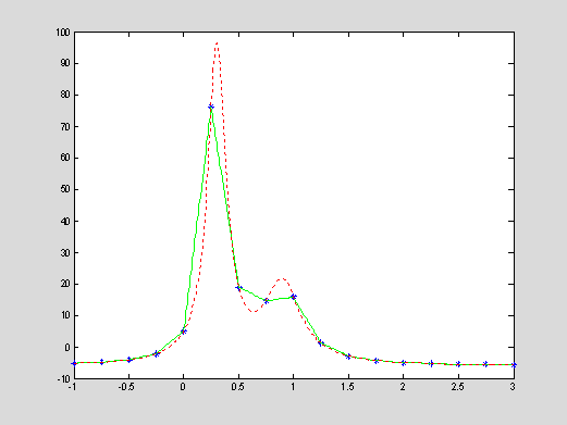
x = -1 : 0.25 : 3; y = humps(x);
n = length(y)-1; a = y(1:n); b =
(y(2:n+1)-y(1:n))./(x(2:n+1)-x(1:n));
% evaluation of linear interpolants at data points xInt
xInt = -1 : 0.01 : 3;
for j = 1 : length(xInt)
if xInt(j) ~= x(n+1)
iInt(j) = sum(x <=
xInt(j));
else
iInt(j) = n;
end
end
yInt = a(iInt) + b(iInt).*(xInt-x(iInt));
yEx = humps(xInt);
plot(x,y,'b*',xInt,yInt,'g',xInt,yEx,'r:'); axis([-1,3,-10,100]);
Cubic
spline interpolation:
Two
consecutive data points (xj,yj) and (xj+1,yj+1)
can be connected by a cubic polynomial:
y = Sj(x) = aj
+ bj (x - xj ) +cj (x - xj)2
+ dj (x - xj)3
The
cubic spline interpolants y = Sj(x) for 1 ![]() j
j ![]() n connect all (n+1) data points and
they have continuous first and second derivatives at the data points. Cubic
spline interpolants provide the smoothest solution of the interpolation problem
and are suitable for plotting of smooth functions y = f(x) from a
given set of data points.
n connect all (n+1) data points and
they have continuous first and second derivatives at the data points. Cubic
spline interpolants provide the smoothest solution of the interpolation problem
and are suitable for plotting of smooth functions y = f(x) from a
given set of data points.
Problem:
Find
coefficients [aj,bj,cj,dj] of
the cubic spline interpolants from the conditions:
continuity of functions: Sj(xj)
= yj; Sj(xj+1) = yj+1
continuity of slopes: S'j(xj)
= S'j-1(xj)
continuity of second derivatives: S''j(xj)
= S''j-1(xj)
There
are (2n) conditions for continuity of functions, (n-1) conditions
for continuity of slopes and (n-1) conditions for continuity of
second derivatives, i.e. the total number of conditions is (4n – 2). However,
there are (4n) unknown coefficients [aj,bj,cj,dj].
Therefore, two more conditions should be added to the problem. These
two conditions are set at the end points as the natural spline conditions:
S''1(x1)
= 0; S''n(xn+1)
= 0
Solution:
Denote mj
= S''j(xj) and hj = xj+1 -
xj, then two coefficients are found from continuity of
second derivatives:
cj = ![]() and dj
=
and dj
= ![]()
Two
coefficients are found from continuity of functions:
aj = yj
and
bj = ![]() -
- ![]() hj
hj
Thus,
all coefficients are parameterized by values of mj. Those
values are found from continuity of slopes at the (n-1) interior
points. The latter conditions result in a system of (n-1) equations:
hj-1 mj-1
+ 2 (hj-1 + hj) mj + hj mj+1 =
6 ![]()
![]() -
- ![]()
![]() ; j = 2,…,n
; j = 2,…,n
The boundary values for natural splines: m1
= 0 and mn+1 = 0.
The boundary values for not-a-knot (cubic runout) splines:
m1
= (1 + ![]() )m2 –
)m2 – ![]() m3
and mn+1 = (1 +
m3
and mn+1 = (1 + ![]() )mn –
)mn – ![]() mn-1
mn-1
% computation of coefficients of cubic spline interpolants from a
set [x,y]
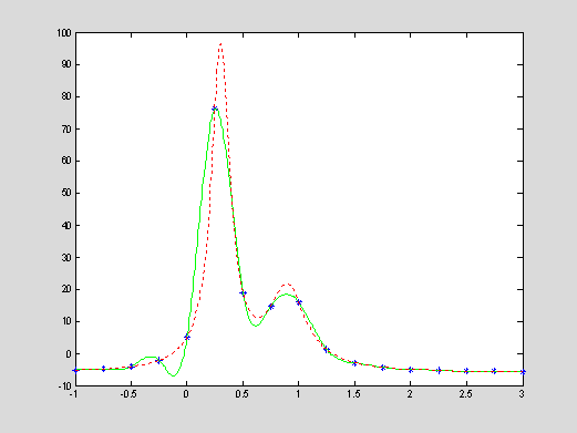
x = -1 : 0.25 : 3; % data partition
y = humps(x); %
function values
n = length(x)-1;
h = x(2:n+1)-x(1:n); % vector of step sizes of the partition of x
A = 2*diag(h(1:n-1)) + 2*diag(h(2:n)) + diag(h(2:n-1),1) +
diag(h(2:n-1),-1);
b = 6*((y(3:n+1)-y(2:n))./h(2:n)-(y(2:n)-y(1:n-1))./h(1:n-1));
m = A\b';
m = [0;m;0]'; % solving the linear system for natural splines
a = y(1:n);
b = (y(2:n+1)-y(1:n))./h(1:n)-h(1:n).*(m(2:n+1)+2*m(1:n))/6;
c = 0.5*m(1:n);
d = (m(2:n+1)-m(1:n))./(6*h(1:n));
% evaluation of cubic spline interpolants at data points xInt
xInt = -1 : 0.01 : 3;
% another partition with better resolution
for j = 1 : length(xInt)
if xInt(j) ~= x(n+1)
iInt(j) = sum(x <=
xInt(j));
else
iInt(j) = n;
end
end
yInt = a(iInt) + b(iInt).*(xInt-x(iInt)) + c(iInt).*(xInt -
x(iInt)).^2 + d(iInt).*(xInt - x(iInt)).^3;
yEx = humps(xInt);
plot(x,y,'b*',xInt,yInt,'g',xInt,yEx,'r:');
axis([-1,3,-10,100]);
Cubic
Hermite interpolation:
Two
consecutive data points (xj,yj) and (xj+1,yj+1)
can be connected by a cubic Hermite polynomial:
y = Sj(x) = aj
+ bj (x - xj ) +cj (x - xj)2
+ dj (x - xj)2 (x - xj+1)
The
cubic Hermite interpolants y = Sj(x) for 1 ![]() j
j ![]() n connect the data points (xj,yj)
with the prescribed slopes sj = y'j at each
data point. Therefore, the cubic Hermite interpolants have continuous first
derivatives at the data points. However, they do not have continuous second
derivatives at the data points. The cubic Hermite interpolation may be too
crude in graphical applications, because the human eye can detect discontinuities
in the second derivative (curvature).
n connect the data points (xj,yj)
with the prescribed slopes sj = y'j at each
data point. Therefore, the cubic Hermite interpolants have continuous first
derivatives at the data points. However, they do not have continuous second
derivatives at the data points. The cubic Hermite interpolation may be too
crude in graphical applications, because the human eye can detect discontinuities
in the second derivative (curvature).
Problem:
Find
coefficients [aj,bj,cj,dj] of
the cubic Hermite interpolants from the conditions:
continuity of functions: Sj(xj)
= yj; Sj(xj+1) = yj+1
continuity of slopes: S'j(xj)
= sj; S'j-1(xj) = sj+1
There
are (2n) conditions for continuity of functions and (2n) conditions
for continuity of slopes, i.e. the total number of conditions is (4n). There
are (4n) unknown coefficients [aj,bj,cj,dj].
Therefore, the problem has a unique solution.
Solution:
At the
left-end point x = xj, we find two coefficients:
aj = yj
and
bj = sj.
At
the right-end point x = xj+1, we find a system of
equations for cj,dj that has a solution:
cj = ![]()
![]()
![]() - sj
- sj![]() and dj =
and dj =![]()
![]() sj+1 + sj - 2
sj+1 + sj - 2![]()
![]()
% computation
of coefficients of cubic Hermite interpolants from a set [x,y]
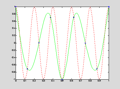
x = 0:0.125:1; % data partition
y = cos(10*pi*x); % function values
s = -10*pi*sin(10*pi*x); % slope values
n = length(x)-1;
h = x(2:n+1)-x(1:n); % vector of step sizes of the partition of x
a = y(1:n);
b = s(1:n);
c = ((y(2:n+1)-y(1:n))./h(1:n)-s(1:n))./h(1:n);
d =
(s(2:n+1)+s(1:n)-2*(y(2:n+1)-y(1:n))./h(1:n))./(h(1:n).^2);
% evaluation of cubic Hermite interpolants at data points xInt
xInt = 0 : 0.01 : 1;
% another partition with better resolution
for j = 1 : length(xInt)
if xInt(j) ~= x(n+1)
iInt(j) = sum(x <=
xInt(j));
else
iInt(j) = n;
end
end
yInt = a(iInt) + b(iInt).*(xInt-x(iInt)) + c(iInt).*(xInt -
x(iInt)).^2 + d(iInt).*(xInt - x(iInt)).^2.*(xInt-x(iInt+1));
yEx = cos(10*pi*xInt);
plot(x,y,'b*',xInt,yInt,'g',xInt,yEx,'r:');
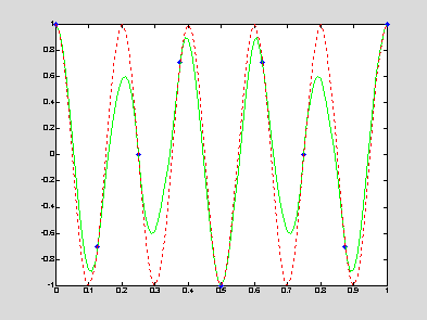
The example above is difficult for interpolation since the function oscillates rapidly and too few data points are given. However, the cubic Hermite interpolation resembles the behaviour of the function. For comparison, below is the result of the cubic spline interpolation on the same data set. Without information about slopes of function at the given data points, the cubic spline interpolation works worse to display the function.
x = 0:0.125:1; y = cos(10*pi*x); n = length(x)-1; h =
x(2:n+1)-x(1:n);
A = 2*diag(h(1:n-1)) + 2*diag(h(2:n)) + diag(h(2:n-1),1) +
diag(h(2:n-1),-1);
b = 6*((y(3:n+1)-y(2:n))./h(2:n)-(y(2:n)-y(1:n-1))./h(1:n-1));
m = A\b'; m = [0;m;0]'; a = y(1:n);
b = (y(2:n+1)-y(1:n))./h(1:n)-h(1:n).*(m(2:n+1)+2*m(1:n))/6;
c = 0.5*m(1:n); d = (m(2:n+1)-m(1:n))./(6*h(1:n));
xInt = 0 : 0.01 : 1;
% another partition with better resolution
yInt = a(iInt) + b(iInt).*(xInt-x(iInt)) + c(iInt).*(xInt -
x(iInt)).^2 + d(iInt).*(xInt - x(iInt)).^3;
yEx = cos(10*pi*xInt);
plot(x,y,'b*',xInt,yInt,'g',xInt,yEx,'r:');