CHAPTER 3: NUMERICAL ALGORITHMS WITH MATLAB
Lecture 3.2: Least square
curve fitting
Polynomial approximation:
Problem: Given a set of (n+1) data points:
(x1,y1);
(x2,y2); …; (xn,yn); (xn+1,yn+1)
Find
a polynomial of degree m < n, y = ![]() m(x), that
best fits to the given set of (n+1) data points.
m(x), that
best fits to the given set of (n+1) data points.
Example:
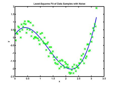
If the data
set is corrupted by measurement noise, i.e. the data values are rounded off,
the numerical interpolation would produce a very stiff curve with sharp corners
and large interpolation error. Another technique is used instead: it is based
on numerical approximation of given data values. The figure below shows
numerical approximation of more than hundred of data values by a cubic
polynomial:
Polynomial
approximation is effective when the data values fit a simple curve, e.g. a
polynomial of lower order. In many cases, the simple (polynomial) curves are
predicted by solutions of theoretical models (e.g. differential equations).
Methods of numerical approximation allow researchers to compare theoretical
models and real data samples.
Methods:
·
Minimization
of total square error
·
Over-determined
linear system
·
MATLAB
"polyfit" functions
Minimization of total square error:
Let
y = ![]() m(x) be a function that best fits to the
given data points in the sense that it minimizes the total square error between
the data points and the values of the function:
m(x) be a function that best fits to the
given data points in the sense that it minimizes the total square error between
the data points and the values of the function:
(min) E = ![]() ( yj -
( yj - ![]() m(xj) )2
m(xj) )2
Linear
regression: y = ![]() 1(x) = c1 x + c2
1(x) = c1 x + c2
Total
error: E = ![]() ( yj – c1 xj – c2
)2
( yj – c1 xj – c2
)2
Minimization:
![]() = -2
= -2 ![]() xj ( yj – c1 xj –
c2 ) = 0
xj ( yj – c1 xj –
c2 ) = 0
![]() = -2
= -2 ![]() ( yj – c1 xj – c2
) = 0
( yj – c1 xj – c2
) = 0
x = [
0.1,0.4,0.5,0.7,0.7,0.9 ]
y = [ 0.61,0.92,0.99,1.52,1.47,2.03]
a11 = sum(x.^2); a12 = sum(x); a21 = sum(x); a22 =
sum(ones(1,length(x)));
A = [ a11,a12; a21,a22]; % the coefficient matrix of the
minimization problem
b1 = sum(x.*y); b2 = sum(y);
b = [ b1; b2 ]; % right-hand-side of the minimization problem
c = A \ b % solution of
the minimization problem
xApr = 0 : 0.001 : 1; yApr = c(1)*xApr + c(2);
plot(x,y,'*g',xApr,yApr,'b');
x = 0.1000 0.4000
0.5000 0.7000 0.7000
0.9000
y = 0.6100
0.9200 0.9900 1.5200
1.4700 2.0300
c = 1.7646
0.2862
Over-determined
linear system:
Suppose
the approximating polynomial y = ![]() m(x) passes through all given points:
m(x) passes through all given points:![]() m(xj) = yj. These
conditions set an over-determined linear system A c = b, when the
number of equations (n+1) exceeds the number of unknowns (m
+1). Since the coefficient matrix A is not singular, no
solution of such over-determined system exists. However, we can still solve the
system in the approximation sense: (A'*A) c = (A'*b). The
coefficient matrix (A'*A) is now 2-by-2 non-singular matrix, such
that a unique solution exists for c. This solution is the same
solution that gives minimum of the total square error E.
m(xj) = yj. These
conditions set an over-determined linear system A c = b, when the
number of equations (n+1) exceeds the number of unknowns (m
+1). Since the coefficient matrix A is not singular, no
solution of such over-determined system exists. However, we can still solve the
system in the approximation sense: (A'*A) c = (A'*b). The
coefficient matrix (A'*A) is now 2-by-2 non-singular matrix, such
that a unique solution exists for c. This solution is the same
solution that gives minimum of the total square error E.
Linear regression: c1 xj + c2 = yj, j = 1,2,…,(n+1)
x = [
0.1,0.4,0.5,0.7,0.7,0.9 ];
y = [ 0.61,0.92,0.99,1.52,1.47,2.03];
A = [ x', ones(length(x),1) ];
% the coefficient matrix of the over-determined problem
b = y'; % right-hand-side of the over-determined problem
c = (A'*A) \ (A'*b) %
solution of the over-determined problem
xApr = 0 : 0.001 : 1; yApr = c(1)*xApr + c(2);

% MATLAB solves the over-determined system in the least square
sense
E = sum((y-c(1)*x-c(2)).^2)
|
A = 0.1000 1.0000 0.4000 1.0000 0.5000 1.0000 0.7000 1.0000 0.7000 1.0000 0.9000 1.0000 |
b = 0.6100 0.9200 0.9900 1.5200 1.4700 2.0300 |
0.2862 E = 0.0856 |
The
total square error E becomes smaller, if the approximating
polynomial y = ![]() m(x) has larger order m < n. The
total square error E is zero, if m = n, i.e. the
approximating polynomial y =
m(x) has larger order m < n. The
total square error E is zero, if m = n, i.e. the
approximating polynomial y = ![]() m(x) is the interpolating polynomial y
= Pn(x) that passes through all (n+1) data
points.
m(x) is the interpolating polynomial y
= Pn(x) that passes through all (n+1) data
points.
x = [
0.1,0.4,0.5,0.7,0.7,0.9 ];
y = [ 0.61,0.92,0.99,1.52,1.47,2.03];
n = length(x)-1;
for m = 1 : n
A = vander(x); A = A(:,n-m+1:n+1);
b = y'; c = A\b; yy = polyval(c,x);
E = sum((y-yy).^2) ;
fprintf('m = %d, E = %6.5f\n',m,E);
end
m = 2; A = vander(x); A = A(:,n-m+1:n+1); b = y';
c = A\b; xApr = 0 : 0.001 : 1; yApr = polyval(c,xApr);
plot(x,y,'*g',xApr,yApr,'b');
m = 2, E = 0.00665
m = 3, E = 0.00646
m = 4, E = 0.00125
Warning: Matrix is singular to working precision.
m = 5, E = Inf
The
system of linear equations for least square approximation is ill-conditioned
when n is large and also when data points include both very small
and very large values of x. Systems of orthogonal polynomials are
used regularly in those cases.
·
polyfit: computes coefficients of approximating polynomial when m < n and
coefficients of interpolating polynomial when m = n
Nonlinear
approximation:
Theoretical dependences fitting data samples can be expressed in terms of nonlinear functions rather than in terms of polynomial functions. For example, theoretical curves can be given by power functions or exponential functions. In both the cases, the axis (x,y) can be redefined such that the linear polynomial regression can still be used for nonlinear least square approximation.
Power function approximation: y = ![]() x
x![]()
Take the logarithm of the power function:
log y = ![]() log x + log
log x + log ![]()
In
logarithmic axis (logx,logy), the data sample can be approximated
by a linear regression.
x =
[0.15,0.4,0.6,1.01,1.5,2.2,2.4,2.7,2.9,3.5,3.8,4.4,4.6,5.1,6.6,7.6];
y =
[4.5,5.1,5.7,6.3,7.1,7.6,7.5,8.1,7.9,8.2,8.5,8.7,9.0,9.2,9.5,9.9];
c = polyfit(log(x),log(y),1) % linear regression in logarithmic
axis
xInt = linspace(x(1),x(length(x)),100);
yInt = exp(c(2))*xInt.^(c(1));
plot(x,y,'g*',xInt,yInt,'b');
% nonlinear regression in (x,y)
loglog(x,y,'g*',xInt,yInt,'b'); % linear regression in (logx,logy)
|
|
|
Exponential function approximation: y = ![]() e
e![]()
Take the logarithm of the exponential function:
log y = ![]() x + log
x + log ![]()
In
semi-logarithmic axis (x,logy), the data sample can be
approximated by a linear regression
Approximation
by a linear combination of nonlinear functions:
y = c1 f1(x)
+ c2 f2(x) + … + cn fn(x)
Trully
nonlinear approximation: y = f(x;c1,c2,…,cn)
It
represents a rather complicated problem of nonlinear optimization.