LAB 7: VOLUME OF A HEART AND LEAST SQUARE APPROXIMATION
Mathematics:
Experimental and numerical data do not generally fit to theoretical dependences because of experimental and numerical errors. If the error of data detection is sufficient small, data points are expected to resemble a theoretical curve. This assumption enables us to approximate parameters of a theoretical formula by computing the least-square approximation between a theoretical curve and real (experimental and numerical) data points. If the theoretical curve is simply a polynomial, the least-square approximation is a polynomial approximation. In many modelling problems, the theoretical curve is however expressed by exponential, logarithmic, power, and trigonometric functions, i.e. the least-square approximation is a nonlinear approximation. This project exploits the least-square approximation with an exponential function for an applicational modelling problem in medical science.
Consider a cardiology research unit that performs an experiment in which a dye is injected at a constant rate into the vein that empties directly into the heart. Small samples of blood are withdrawn at regular intervals from the artery that carries blood directly out of the heart. Concentration of the dye in the heart's blood was found in two trials as a function of time:
Trial I:
|
Concentration |
0.0243291 |
0.0368201 |
0.0465258 |
0.0480842 |
0.0499363 |
|
Time in sec |
2.0 |
4.0 |
8.0 |
12.0 |
20.0 |
Trial II:
|
Concentration |
0.0141734 |
0.031606 |
0.0405562 |
0.0482163 |
0.0496632 |
|
Time in sec |
1.0 |
3.0 |
5.0 |
10.0 |
15.0 |
The mathematical model for concentration of dye in the heart c=c(t) is:
c(t) = rin/rout
(1 – exp(-routt/V))
where V is the volumne of the heart in mL,
rin is the total amount of dye pumped in the heart per
second, and rout is the total amount of blood pubped
out of the heart per second. We assume rin = 5
mL/sec and rout = 100mL/sec. In
order to determine V, we have a set of five data points (tk,ck)
and fixed values for parameters rin and
rout. By regrouping terms of the formula for c(t) and
taking a logarithm, we reduce the formula for c(t) to a linear
formula for t = t(c):
t = - V*log(1 – rout c/rin) / rout
The linear least-square approximation can now be used to
find a value for V from the two sets of five data points for t
versus d = log(1 – rout c / rin ).
|
|
|
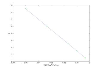
The first data set
results in the least square approximation for the volume of a heart: V = 311.25 ml with the total square error E = 4.09. The second data set
results in the least square approximation V = 299.99 ml with
the total square error E = 0.00. Therefore, the second data set is more
accurate for the theoretical dependence c = c(t).
Objectives:
·
understand
the computational algorithm for nonlinear least-square approximations
·
exploit
linear least-square approximations by solving a linear over-determined system
·
exploit
MATLAB polynomial functions and least-square approximations
MATLAB script for least square approximations by solving a linear over-determined system:
t = - V*d, d = log(1 – rout c/rin)
/ rout
Steps
in writing the MATLAB script:
- Define parameters rin
= 5 and rout = 100.
- Define the given set of
five data points for t and c.
- Compute the vectors for
d = log(1 – rout c / rin ) / rout.
- Set up a coefficient
matrix A for an over-determined linear system: A V = t.
- Solve the
over-determined linear system for V
in the sense of a linear
least-square approximation. Display the value for V.
- Comute the total square error E of the linear least-square approximation. Display the value for E.
- Plot the data points
and the linear least-square approximation on the plane (d,t).
- Plot the data points
and the nonlinear least-square approximation on the plane (t,c).
Exploiting
the MATLAB script:
- Compute the
least-square approximations for the two data sets.
- Which data set is more
accurate? Compare the total square error and the graphs of least-square
approximations versus the data points.
MATLAB script for least square approximations by using MATLAB polynomial functions:
t = a1(-d) + a2, a1 = V, a2 = t0, d = log(1 – rout c/rin)
/ rout
Steps
in writing the MATLAB script:
- Steps (1)-(3) of the
first script.
- Use "polyfit"
to find the linear least square approximation for the data (d,t).
- Compute the value for V and the total square error E.
- Use "polyval" to compute and plot the linear least square approximation on the
plane (d,t).
- Plot the data points
and the nonlinear least-square approximation on the plane (t,c).
Exploiting
the MATLAB script:
- Compute the
least-square approximations for the two data sets for t and c.
- Which data set is more
accurate? Compare the intercepts t0 of the linear
least-square approximation on the plane (d,t) with that
prescribed by the theoretical formula.
- Compare graphs of
least-square approximations obtained in the first and in the second
scripts.
QUIZ "Evolution of statistical parameters in a random walk of molecules (diffusion)":
Consider
the same problem as in Script #2 of Lab. # 2, i.e. the random
walk of N molecules after n collisions. The
diffusion theory predicts that![]() = 0 and
= 0 and ![]() 2 = D n, where D is
diffusion coefficient,
2 = D n, where D is
diffusion coefficient, ![]() is the mean and
is the mean and ![]() 2 is the variance:
2 is the variance:
![]() =
= ![]()
![]() xk(n),
xk(n),
![]() 2 =
2 = ![]()
![]() ( xk(n) -
( xk(n) - ![]() )2
)2
Evolution
of the mean![]() and the variance
and the variance![]() 2 in time n depends on the
number of molecules N in a statistical ensemble, as well as on
each particular random data realization. A typical pattern for evolution of the
mean
2 in time n depends on the
number of molecules N in a statistical ensemble, as well as on
each particular random data realization. A typical pattern for evolution of the
mean![]() and the variance
and the variance![]() 2 for 10 different ensembles
with different values of N is shown here:
2 for 10 different ensembles
with different values of N is shown here:
|
|
|
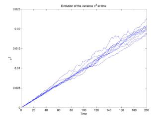
The
coefficient of diffusion D can be computed as the slope of the
least-square approximation of the curve![]() 2 in time n. The basic
script with computations of
2 in time n. The basic
script with computations of ![]() and
and ![]() 2 is attached. Continue the script and
compute the coefficient of diffusion for an ensemble of N = 500 molecules.
2 is attached. Continue the script and
compute the coefficient of diffusion for an ensemble of N = 500 molecules.