LAB 6: THREE-DIMENSIONAL GRAPHICS AND CURVILINEAR GRIDS
Mathematics:
A function of two
variables u = f(x,y) is plotted as a surface in a space of three
dimensions (x,y,u). When a rectangular domain of (x,y) is divided into sets of rectangles at the grid points in x and in y , the function u = f(x,y) is
defined on the rectangular (Cartesian) grid. Other curvilinear grids are also used
in various problems due to symmetries of the function f(x,y), symmetries of the domain of (x,y),
or for a better design of numerical
algorithms. This project is to study plotting of three-dimensional surfaces on
the circular and triangular (curvilinear)
grids.
MATLAB
three-dimensional graphics can be used for functions defined at the curvilinear
grids. If (xi,j,yi,j)
are matrices for the
coordinates of the curvilinear grid points, the function u = f(x,y) is defined as the matrix
ui,j = f(xi,j,yi,j). Provided that the sizes of these three
matrices agree, contour plots, mesh surfaces and painted surfaces with lighting
can be constructed for functions defined at the curvilinear grids.
Objectives:
·
Understand
methods of building grid matrices (xi,j,yi,j)
from coordinates of the curvilinear grid points.
·
Exploit
visualization of surfaces with circular symmetry.
·
Exploit
visualization of surfaces defined at the triangular grids.
MATLAB script for plotting functions on a circular grid:
When the function u = f(x,y) has a circular symmetry and is defined in a
disk or in an annulus, it is convenient to locate the grid points at circles of
radius r. The function u = f(x,y) can be
rewritten as the function u =
u(r,![]() ) in polar
coordinates:
) in polar
coordinates:
x = r*cos(![]() ), y = r*sin(
), y = r*sin(![]() ),
),
where r is radius from (x,y) to the origin (0,0) and ![]() is the angle between
the vector (x,y) and the positive x axis. For example,
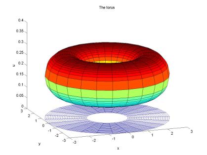
the torus is defined by the function:
is the angle between
the vector (x,y) and the positive x axis. For example,
the torus is defined by the function:
u = ![]() (R2 – (r-a)2)1/2 for a-R
(R2 – (r-a)2)1/2 for a-R ![]() r
r ![]() a+R,
a+R,
where a > R. The circular grid for the torus and the
surface in the space (x,y,u) are shown here:
Steps
in writing the script:
- Define the grid for
radius vector r between [a-R,a+R] for R
= 1 and a = 2.
- Define the grid for
angle vector theta between [0,2*pi].
- Compute the matrices xi,j
and yi,j in polar coordinates. Use
the outer products of vectors r and
 .
. - Open window #1 and plot
the circular grid alone.
- Compute the matrix ui,j
for each grid point on the circular grid.
- Open window #2 and plot
the contour plots of the torus between u = 0 and u = umax.
- Open window #3 and plot
the surface for the torus. Display positive and negative values of u
at the same graph. Draw the surface and the circular grid at the
same graph.
Exploiting
the MATLAB script:
- Use surface with
lighting for the following colormaps: hot, cold, jet, grey. Observe the difference in
visualization of the surface.
- Use surface with
lighting for the following shadings: flat, interp. Observe the
difference in visualization of the surface.
- Change view of the tour
by rotating the graph with view.
MATLAB script for plotting functions on a triangular grid:
When the function u = f(x,y) is computed as solution of a boundary value
problem based on finite element methods, the function is usually defined on a
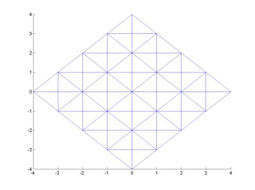
triangular grid, that consists of triangular elements. An example of a
triangular grid consisting of 64
triangles and 41 vertices (nodal points) is shown here:
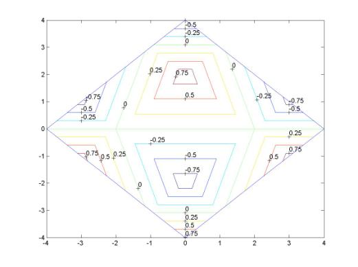
Suppose the
function u = f(x,y) =
cos(x)*sin(y) is computed in
the vertices of the triangular grid (e.g. with the use of the finite-element
method). When the numerical approximation of the function u = f(x,y) is known at the vertices, the contour plot
and the surface can be computed in the given domain of (x,y). The contour plot of the function looks like:
Steps
in writing the script:
- Define a structure for
two coordinates of each vertex (nodal point) on the triangular grid.
- Define a structure for
three vertex point numbers of each triangular element of the triangular
grid.
- Open window #1 and plot
the triangular grid alone.
- Build the matrices (xi,j,yi,j) for coordinates of the triangular grid.
- Compute the matrix ui,j
for each grid point at the triangular grid.
- Open window #2 and plot
6 contour plots of the function u
= f(x,y). Draw the
boundary of the domain at the same graph.
- Open window #3 and plot
the surface for the function u =
f(x,y). Display positive and negative values of u at
the same graph. Draw the surface and the grid at the same graph.
Exploiting
the MATLAB script:
- Construct the same
function u = f(x,y) =
cos(x)*sin(y) on a rectangular grid between –4
 x
x  4 and -4
  y
y  4 with
step-size 1.
4 with
step-size 1. - Draw the contour plot and the surface as in steps (6)-(7). Compare
the approximation of the function on rectangular and triangular grids.
QUIZ:
- Plot the sausaged torus
defined in polar coordinates:
u = ![]() (R2 – (r-a)2)1/2*cos(3
(R2 – (r-a)2)1/2*cos(3![]() ) for a-R
) for a-R ![]() r
r ![]() a+R
a+R
- Plot the lump soliton
in the disk of radius 4 by using polar coordinates:
u = (1 + y2 – x2)/(1 + x2
+ y2)2