LABORATORY 2: RANDOM WALKS AND MONTE-CARLO SIMULATIONS
Mathematics:
A molecule moves as a result of collisions
with other molecules. Suppose an average time between two collisions equals to![]() t = 1. Also suppose that a single collision displaces a
molecule by
t = 1. Also suppose that a single collision displaces a
molecule by ![]() x = s in the direction of the x-axis or
in the opposite direction. If collisions are equally likely in both directions,
the probabilities of the molecule's shift to the right and to the left after an
individual collision are the same: p = q = ½. This is the
simplest model for a one-dimensional random walk of molecules called the Brownian
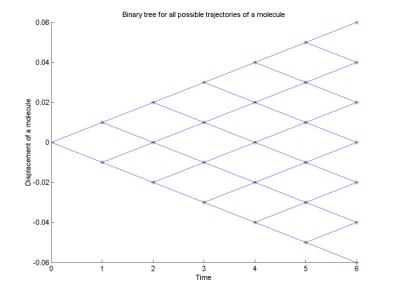
motion. If x is a position of a molecule, then all possible
moves (trajectories) of x as a result of n
collisions with other molecules are shown on the picture called a binary
tree (shown for n = 6):
x = s in the direction of the x-axis or
in the opposite direction. If collisions are equally likely in both directions,
the probabilities of the molecule's shift to the right and to the left after an
individual collision are the same: p = q = ½. This is the
simplest model for a one-dimensional random walk of molecules called the Brownian
motion. If x is a position of a molecule, then all possible
moves (trajectories) of x as a result of n
collisions with other molecules are shown on the picture called a binary
tree (shown for n = 6):
Consider
an ensemble of N molecules thrown in a single point, say x = 0. As
a result of molecular collisions, they start to spread or to diffuse. Let xk(n)
denote a displacement of the k-th molecule after n
collisions. The diffusion (spread) of molecules can be characterized by two
mathematical quantities:
·
mean (average
displacement): ![]() =
= ![]()
![]() xk(n)
xk(n)
·
variance (average squared displacement):![]() 2 =
2 = ![]()
![]() ( xk(n) -
( xk(n) - ![]() )2
)2
The
theory of diffusion works for large N and predicts that ![]() = 0 and
= 0 and ![]() 2 = D n, where D is the
coefficient of diffusion.
2 = D n, where D is the
coefficient of diffusion.
Objectives:
·
visualize
individual trajectories of molecules in the ensemble of N molecules
·
plot
the mean![]() and the variance
and the variance![]() 2 as functions of n for an
ensemble of N molecules and find the coefficient of diffusion D
2 as functions of n for an
ensemble of N molecules and find the coefficient of diffusion D
·
plot
the mean![]() and the variance
and the variance![]() 2 as functions of N for the same number of n collisions and
compare with the theoretical values for
2 as functions of N for the same number of n collisions and
compare with the theoretical values for![]() and
and![]() 2
2
·
understand
limits of applicability of the theory of diffusion
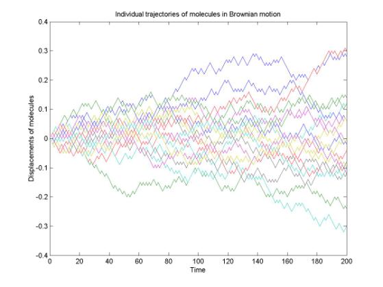
MATLAB script "Individual trajectories of molecules in Brownian motion"
A
typical pattern of N = 15 molecules for n = 200 collisions
is shown here:
Steps in writing the MATLAB script:
- Initialize values of s, N, and n.
- Create a matrix of N by n random numbers equally distributed in the interval [-0.5, 0.5].
- Transform the entries of the random matrix to the binary entries: +s and –s.
- Compute an N by
n matrix of total displacements of molecules by summing
columns of the binary matrix in (3) between the first column (a starting
time of collisions) and an intermediate column (the current time of
collisions).
- Plot each row of the
matrix of total displacements at the same graph.
Exploiting
the MATLAB script:
- Run the script with N
= 10; 20; 50 and n = 100; 200; 300.
- Check that the
trajectories are more spreaded for larger values of n
- Check that the
trajectories are symmetric about the zero mean for large values of N
MATLAB script "Evolution of statistical parameters in a random walk of molecules (diffusion)"
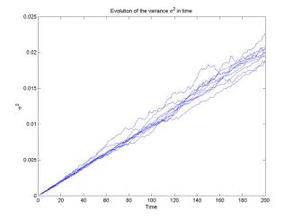
The
diffusion theory predicts that the mean ![]() stays at zero
in time (with larger number of collisions n), while the variance
stays at zero
in time (with larger number of collisions n), while the variance![]() 2 grows linearly in time. Evolution of the
mean
2 grows linearly in time. Evolution of the
mean![]() and the variance
and the variance![]() 2 in time depends on the number of
molecules N in a statistical ensemble, as well as on each
particular random data realization. Such numerical computations are called the
Monte-Carlo simulations. A typical pattern for evolution of the mean
2 in time depends on the number of
molecules N in a statistical ensemble, as well as on each
particular random data realization. Such numerical computations are called the
Monte-Carlo simulations. A typical pattern for evolution of the mean![]() and the variance
and the variance![]() 2 is shown here for ten ensembles with
different values of N.
2 is shown here for ten ensembles with
different values of N.
|
|
|
We
can compute the coefficient of diffusion D (the slope of the line![]() 2 versus time) and plot it as functions of
number of molecules N. The theory predicts that the Monte-Carlo
approximation of D should approach to the theoretical value of D with large N.
2 versus time) and plot it as functions of
number of molecules N. The theory predicts that the Monte-Carlo
approximation of D should approach to the theoretical value of D with large N.
|
|
Steps in writing the MATLAB script:
|
Exploiting
the MATLAB script:
- Run the script with the
same values of N = 100 : 100 : 1000 and n = 200
several times and check that each time Monte-Carlo simulations produce a
different but similar picture.
- Comment the part of the
script where plots of figure(1) and figure(2) are computed (this operation
takes a lot of computational time). Run the script for N = 500 : 500 :
10000. Is there a better convergence for the coefficient of diffusion D
as a function of N?
QUIZ: MATLAB script "Comparison of the average theory with individual trajectories of molecules"
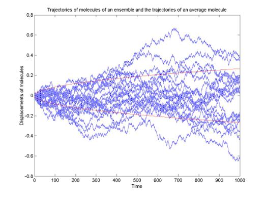
The
theory predicts that the standard deviation of an average molecule grows as a
parabola with respect to time: ![]() =
= ![]() Due to the symmetry,
molecules spread to the left and to the right equally likely. We can combine
the parabolic walk of an average molecule in time with individual random
trajectories of molecules in a given ensemble. A typical pattern for N =
20 and n = 1000 is shown here:
Due to the symmetry,
molecules spread to the left and to the right equally likely. We can combine
the parabolic walk of an average molecule in time with individual random
trajectories of molecules in a given ensemble. A typical pattern for N =
20 and n = 1000 is shown here:
Steps in writing the MATLAB script:
1.
Compute
the random matrix of total displacement similar to the first script
2.
Compute
the mean, variance, and the coefficient of diffusion similar to the second script.
3.
Plot
each row of the matrix of total displacements at the same graph by blue color.
4.
Compute
two vectors for positive and negative trajectories of an average molecule.
5.
Plot
the two vectors at the same graph by red color.
Exploiting
the MATLAB script:
- Run the script with N
= 20; 50 and n = 200; 500.