LAB 10: AGE-SPECIFIC POPULATION GROWTH AND MATRIX EIGENVALUES

Mathematics:

Demographic predictions of population growth are based on a number of mathematical models. This project exploits the Leslie matrix model, where the female population is divided into age classes of equal duration. As time progresses, the number of females, within each class, changes because of birth, death, and aging.

Suppose we study n age classes of females over maximum age in T years and denote the number of females in the j-th class at the k-th time instance by x_j^(k). Each age class is T/n years in duration. It makes sense therefore to study changes of the number of females x_j^(k) between two observation times in T/n years. All females of the j-th class at the k-th time pass into the (j+1)-th class at the (k+1)-th time, except for those who died during the time interval. Denote b_j be the fraction of females that survives in the j-th class, i.e.0 b_j 1 and

x_j+1^(k+1) = b_j x_j^(k), j = 1,2,…,n-1

The first class at the (k+1)-th time has the number of females x₁^(k+1) that was born during the time interval by females of all other classes. Denote a_j be the average number of daughters born by each female in the j-th class during the time inteval, i.e. a_j 0 and

x₁^(k+1) = a₁ x₁^(k) + a₂ x₂^(k) + … + a_n x_n^(k)

The following birth and death parameters were registered from the year 1965 for Canadian females:

Age	[0,5)	[5,10)	[10,15)	[15,20)	[20,25)	[25,30)	[30,35)	[35,40)	[40,45)	[45,50)
aj	0.00	0.00024	0.05861	0.28608	0.44791	0.36399	0.22259	0.10457	0.02826	0.00240
bj	0.99651	0.99820	0.99802	0.99729	0.99694	0.99621	0.99460	0.99184	0.98700	---

In this table, the age classes over T = 50 years are neglected since they rarely have children, i.e. a_j = 0 , j > n, where n = 10 age classes with duration in T/n = 5 years.

Introducing matrix notations, the Leslie model can be written as the discrete dynamical system x^(k+1) = L x^(k), where x^(k) is age distribution vector at the k-th time and L is the Leslie matrix:

L =

The Leslie matrix L is supposed to have at least two non-zero successive entries a_j and a_j+1. The matrix L has n eigenvalues ₁,…,_n with n eigenvectors z₁,…,z_n, such that Lz_j =_j z_j. It can be shown that there is unique positive eigenvalue ₊ which is dominant, i.e. all other negative and complex eigenvalues have smaller absolute value: |_j | < ₊. Let z₊ be the eigenvector for the eigenvalue _+. Then, the long-term behaviour of the age distribution of the female population is:

x^(k) = c ₊^k z₊

The population increases if ₊ > 1, decreases if ₊ < 1 and stabilizes if ₊ = 1.

Objectives:

· Understand the long-term behaviour of the female population within the Leslie model

· Exploit dynamical modeling of the population growth within the Leslie model

· Exploit the power method for finding the dominant eigenvalue and its eigenvector of the matrix L

MATLAB script for dynamical modeling of the population growth within the Leslie model

If Canadian women continued to reproduce and die as they did in 1965, the dynamical growth of female population in the ten age classes every five years would follow this graph:

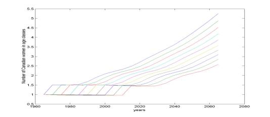
Every five years, the increase in the number of females at each age class, defined as y_j^(k+1) = (x_j^(k+1) – x_j^(k))/x_j^(k), will approach to a uniform ratio for large k, which is approximately 0.07622 or 7.622%. In the year of 2040, the histogram of population is distributed according to the graph:

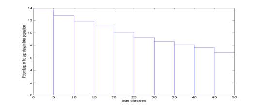
If the vector x^(k) is normalized such that x₁^(k) = 1, the vector x^(k) approaches approximately for large k:

Age class	[0,5)	[5,10)	[10,15)	[15,20)	[20,25)	[25,30)	[30,35)	[35,40)	[40,45)	[45,50)
Proportion	1.000	0.9259	0.8588	0.7964	0.7380	0.6836	0.6328	0.5848	0.5390	0.4943

Steps in writing the MATLAB script:

1. Define T = 50, n = 10, and dT = L/n. Define vectors a and b for the birth and death parameters.
2. Initialize the Leslie matrix L from given vectors a and b.
3. Define the initial age distribution vector x⁽⁰⁾ as vector of ones.
4. Organize a loop and compute the age distribution vector x^(k) for k = 1,2,…,20. Save the results into a matrix X.
5. Plot dynamics of each age class in time. Scale the time axis t starting with 1965 for k = 0.
6. Compute the yield vector y_j^(k) and save the results into a matrix Y.
7. Plot the increase in the number of females of each age class in time t.
8. For the year of 2040, compute the histogram of population at each age class.
9. Normalize the vector x^(k) for the year 2040 such that x₁^(k) = 1. Compare x^(k) with the table above.

MATLAB script for finding the dominant eigenvalue and its eigenvector of the Leslie matrix

Suppose that the Leslie matrix L is diagonalizable, i.e. the eigenvectors z_j can be combined into matrix P:

P = [ z₁, z₂, …, z_n ]

and eigenvalues _j are combined into matrix D = diag[_{1, 2 , …, n}] such that L = P D P^-1. Then, the age distribution vector x^(k) at the k-th time is:

x^(k) = L^k x⁽⁰⁾ = P D^k P^-1 x⁽⁰⁾

If the unique positive eigenvalue₊ is dominant, i.e. all other eigenvalues satisfy: |_j | < ₊, then the age distribution vector x^(k) has the limiting behavior in the limit k :

x^(k) c z₊

where z₊ is the eigenvector for ₊ and c is a constant.

The dominant eigenvalue ₊ and its eigenvector z₊ can be found in the iterative power method based on the asymptotic limit above. Construct a sequence:

x^(k) x^(k+1) = L x^(k)

where c_k = max_j | L x^(k) |_j, i.e. the largest entry in the vector x^(k+1) is normalized by 1. Then, the sequence converges to the eigenvector z₊, while the normalization constant c_k converges to ₊. The dominant eigenvalue for the problem is ₊ = 1.07622 and the eigenvector z₊ is given in the table:

Age class	[0,5)	[5,10)	[10,15)	[15,20)	[20,25)	[25,30)	[30,35)	[35,40)	[40,45)	[45,50)
Eigenvector	1.000	0.9259	0.8588	0.7964	0.7380	0.6836	0.6328	0.5848	0.5390	0.4943

Steps in writing the MATLAB script:

1. Initialize steps (1)-(3) as in the first script.
2. Use MATLAB function "[P,D] = eig(L)" to find the matrix of eigenvectors P and the diagonal matrix of eigenvalues D. Identify the unique positive eigenvalue ₊ and confirm that it is dominant. Compare the corresponding eigenvector z₊ with the one given above.
3. Write a loop for finding x^(k+1), normalizing the maximal element of the vector x^(k+1) by one.
4. Run the loop for 20 values and see how close the normalization constant c_k approaches the dominant eigenvalue _+.
5. Check how close the vector x⁽²⁰⁾ approaches the eigenvector z₊.

Exploiting the MATLAB script:

1. Design termination of the loop when a required criterion of accuracy of the dominant eigenvalue is reached. For example if the difference |c_k+1 – c_k | < tol for any given tolerance tol, an infinite loop can be terminated.

QUIZ:

1) The value of the dominant eigenvalue₊ is determined by the net reproduction rate of the population:

R = a₁ + a₂ b₁ + a₃ b₁ b₂ + … + a_n b₁ b₂ … b_n-1

If R > 1, the population increases. If R < 1, the population decreases. If R = 1, the population stabilizes. Write a function "[R,status] = NetRate(a,b)" that computes the scalar R from the vectors a and b and states in the string status whether the population increases, decreases or stabilizes.

2) Consider the birth-death parameters for the animal population:

Age	[0,5)	[5,10)	[10,15)
aj	0	4	3
bj	0.5	0.25	---

Find the net population growth for the animal population and state whether it increases, decreases, or stabilizes. Compute the dynamics of the animal population in time and confirm the prediction.